NETWORKDAYS Formula in Excel

In Excel, the NETWORKDAYS formula is used to calculate the number of workdays between two dates. The number of weekends is automatically omitted when using the NETWORKDAYS function. It also permits us to exclude certain holidays and only count business days. It is classified as a Date/Time Function in Excel. This formula can be used in Excel to compute working days between two dates.

There are three parameters or arguments of the NETWORKDAYS function: start date, end date and holidays. Valid Excel dates must be used in all three arguments. Holidays parameter are optional. Provide a valid Excel date range for the holidays argument to exclude holidays. Holidays are considered non-working days and are excluded from the calculation.

When determining workdays, NETWORKDAYS considers both dates; the start date and end dates. If the start date and end date are the same, and the date is not a weekend or holiday, then NETWORKDYS will return 1.

For Example, a NETWORKDAYS formula can be written in the following format:

=NETWORKDAYS(start,end) //exclude weekends
=NETWORKDAYS(start,end,holidays) //exclude weekends + holidays

WORKDAYS and NETWORKDAYS are two functions in Microsoft Excel that are precisely developed for calculating weekdays.

The WORKDAY function returns a date N working days in the future or past. We can use the WORKDAY function in order to add or subtract workdays to a given date.

With the help of the NETWORKDAYS function, we can determine the number of workdays between the two dates that we specify.

Syntax of the NETWORKDAYS function

The following is the syntax of the NETWORKDAYS function:

NETWORKDAYS( start_date, end_date, [holidays])

Arguments or Parameters

• start_date:- start_date is a required argument which represents the start date.
• end_date:- end_date is also a required argument which represents the end date
• holidays:- This argument is optional. It is a list of holidays that should be excluded from the computation of working days. It can be entered as a range of cells containing the holiday dates (for example, F2:F5) or a list of serial numbers representing the holidays dates.

Functions of NETWORKDAYS in Excel

• NETWORKDAYS determines the total number of working days between two dates.
• NETWORKDAYS calculates the whole workdays and ignores any time values.
• If we used with the INTL function then it gives the system more flexibility.
• It automatically excludes weekends (Saturday and Sundays) and also allows holidays to be omitted.

Applications of NETWORKDAYS Function

We can use the NETWORKDAYS function for numerous purposes. For example, we can use this function to determine the employee's benefits on the basis of the workdays, the workdays required to resolve a custom support issue, the total days needed to complete a project, etc.

The following are some applications of the NETWORKDAYS formula in Excel spreadsheets:

• Calculates workdays per month
• Calculates the work hours between dates
• Count the total number of business days
• Calculate the number of working days left in a month

Output of the NETWORKDAYS Function

A start date and end date are required for the NETWORKDAYS function to work. The following are the values returned by the NETWORKDAYS function:

• The NETWORKDAYS function returns a positive value if the start date comes before the end date.
• The NETWORKDAYS function returns the value 1 if the start date and end date are the same.
• The NETWORKDAYS function returns a negative value if the end date comes before the start date.
• The function returns a #VALUE! Error if any of the arguments are not recognized by Excel as valid dates.

How to Use the NETWORKDAYS Function in Excel?

Consider the following examples to understand better how the NETWORKDAYS function works.

Example 1: Suppose we need to calculate the working days or business days from January 1, 2021 to January 1, 2022. The holidays in between are:

• March 29, 2021- Holi
• November 4, 2021-Diwali
• December 25, 2021 Christmas Day

We will use the following function in order to calculate the number of working days.

=NETWORKDAYS(A4,B4,C4:C6)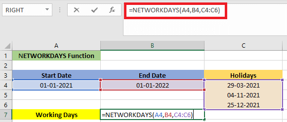

After applying the above formula, we will get the number of working days which is 259, as we can see in the below screenshot.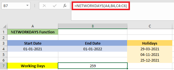

Example 2: Calculate the number of days between two dates (excluding weekends)

As shown in the screenshot below, the start dates are in the range A2:A3, and the end dates are B2:B3. We have to follow the steps below to calculate only working days between the start and end dates and automatically excluding weekends:

1. First, we have to select the cell where we want to display the total number of working days. To do this, we will use the below formula.

=NETWORKDAYS(A2,B2)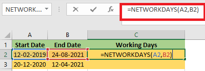

2. After applying the formula, we have to press Enter so that we can get the output.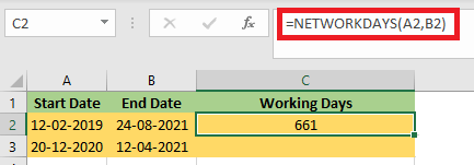

3. Keep selecting the result cell and drag the Fill Handle down to apply the formula to other cells, to calculate the value for the remaining cell.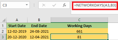

Now the number of working days between the specified start date and end date is calculated.

Example 3: Calculating the Numbers of Days Between Two Dates (Excluding Weekends and Holidays)

If we also want to exclude certain holidays, then the method described in this section can help.

1. Select the cell where we want to show the total number of working days. To do this, we will use the below formula.

=NETWORKDAYS(A2,B2,D2:D3)

In this formula, D2:D3 is the list of holidays we will exclude form the working days.

2. After applying the formula, we have to press Enter so that we can get the output.

3. Keep selecting the result cell, then drag the fill handle to apply the formula to the remaining cells to calculate the value of the remaining cell.

Key Takeaways

• In Excel, the weekend (Saturday and Sunday) is automatically excluded from the
• We can calculate the workdays only if the start date and finish date are specified.
• If the cell format is changed to "General," the numeric value of serial dates can be seen,
• The holidays can be excluded from the total workdays at the option of the Excel user.
• With the help of the NETWORKDAYS function, we can determine the total number of working days between two dates.
• Saturday and Sunday are considered weekends. Use INTL if we want to utilize different days as the weekend.
• If any of the parameters includes an invalid date, then the #VALUE! Error value will be returned.
• The NETWORKDAYS function ignores any time values when calculating working days.
• When computing workdays, the NETWORKDAYS function will take into account both the start and end dates. As a result, if we give NETWORKDAYS the same start and finish dates, it will return