Index function in ExcelWhat is INDEX function?The INDEX function within a table is used to return a value or the reference value in the given range or array. It means that there are two formats of the INDEX function. It is given as:
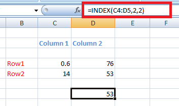
Array formatThe array format is used when we want to return a value of a specified array. The formula of the array format is given by: INDEX(array, row_num, [col_num]) Where, Array: It is the specified array of cells. row_num: It denotes the number of rows in an array of cells. col_num: It denotes the number of columns in the array of cells. Column number of the INDEX function is optional. It can be set to zero or back if there is no requirement of the column in the function. Reference formatThe array format is used when we want to return a value with the reference of the cell. The formula of the reference format is given by: INDEX(reference, row_num, [col_num], [area_num]) Where, Reference: It is the reference of one or more cells in the function. We can insert single or multiple areas directly into the function. But, the individual areas should be enclosed in the brackets and separated by the commas. row_num: It denotes the number of rows in an array of cells. col_num: It denotes the number of columns in the array of cells. area_num: The area number indicates a particular range to use from the multiple ranges specified in the INDEX function. The INDEX function is not same as the vlookup function in excel. But, we can say that it can be used as an alternative way in place of the vlookup command. The Purpose of using the INDEX functionWe have discussed the index function and its two formats. But, it is used for which purpose? The index function is used to find a particular value in a list of tables. Inside the function, we can specify the position of the value that needs to be located because it is difficult to locate a particular value in a table with large data. What value do the INDEX() returns?The INDEX function returns the value at a specified location. It means that whatever location we have declared inside the function (such as row number, column number) will return the specified location's value. How INDEX function works?Let's discuss it with the help of an example. Consider the below table. 
Let find the value 53 from the given table. The steps are as follows:
Similarly, other values of the table can be represented as:
Value = 0.6 Intersection of row1 and column1
Value = 76 Intersection of row1 and column2
Value = 14 Intersection of row2 and column1 If there is cell space between the two rows and columns, it will be considered as a blank row or column. So, we need to count that row and column also. For example, 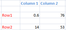
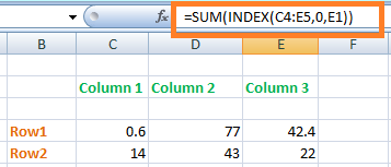
The above table has two columns and three rows. It is because of the one cell space between the two columns and rows, which is considered by default. Hence, we should avoid spaces in between. INDEX function can be used to restore individual values or the entire row or column. We will discuss the examples later in the topic. Relation between INDEX and SUM functionAs discussed, the INDEX function is used to find a value in the given array or table. The SUM function is used to calculate the sum of the specified values. But, what is the relation between these two? The INDEX function declared inside the SUM function can calculate the sum of the value specified in the declared row or column. It is given by: SUM( INDEX (reference, row_num, [col_num]) Let's discuss an example. Consider the below table. 
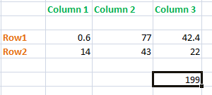
Here, we will calculate the sum of all the numbers present in the table. Consider the below steps:
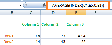
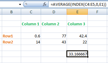
Relation between AVERAGE and INDEX functionAverage is the common word that we have been studying since many years. Average is defined as the division of sum of all the values with the number of values. It is given by: Average = Sum of all the values/ No. of values In excel, we will directly declare AVERAGE function with the INDEX function to compute the average of the specified values. Now, let's consider the same table as of SUM. It is given below: 
Here, we will find the AVERAGE of all the values given in the table. Consider the below steps:
Important pointsPoints to remember before proceeding with INDEX formulas and examples
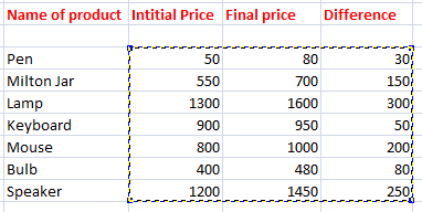
ExamplesLet's discuss some examples for better understanding of the index function. Example 1: To find the final price of lamp.Consider the below table in excel. 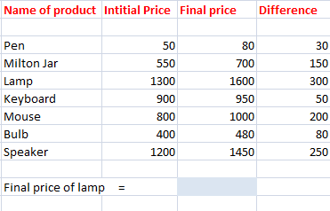
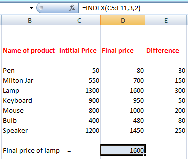
We need first to reconsider the position of the lamp in the given table. The position of the final price column is two, and the lamp's position is row three. The position is according to the selected reference data. Thus, the resulted value will arise from the intersection of the third row and the second column. Let's implement with the help of INDEX function in excel. The steps are as follows:
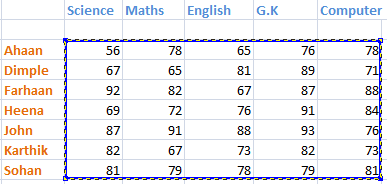
Example 2: To find the sum of the values in the third row and second column separately.Consider the below table. 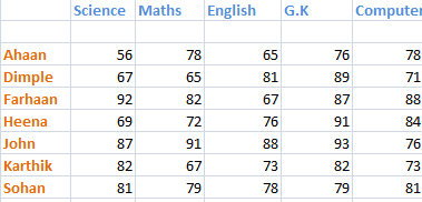
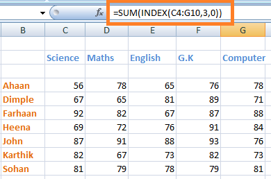
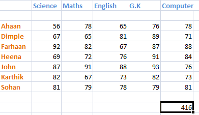
Method 1: To find the sum of the values present in the third row. The third row in the table is shown below: 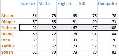
Consider the below steps:
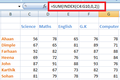
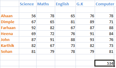
We can verify the sum using the summation symbol on the toolbar. Method 2: To find the sum of values present in the second column. Consider the below steps: The second column in the table is shown below: 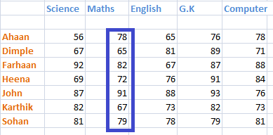
Consider the below steps:
Next TopicHow to remove formula in Excel
|
 For Videos Join Our Youtube Channel: Join Now
Feedback
- Send your Feedback to [email protected]
Help Others, Please Share


