How to Delete Duplicate Rows in ExcelMicrosoft Excel is primarily a calculation tool, and its sheets are often used as databases to keep track of inventories, make sales reports or maintain mailing lists. A common problem that occurs as a large database is that many duplicate rows appear when working with spreadsheets and creating multiple copies of the same document to the same person or calculating the same numbers more than once in a summary report. This can be a very mindless, repetitive, time-consuming task, but several methods for identifying and deleting duplicate rows in Excel make it simpler. Use conditional formatting to find and highlight duplicate data. That way, you can review the duplicates and decide if you want to remove them. Step 1: Select the cells you want to check for duplicates. Step 2: Go to the Home tab and click on the Conditional Formatting. Step 3: go to the Highlight Cells Rules and click on the Duplicate Values in the drop-down list. 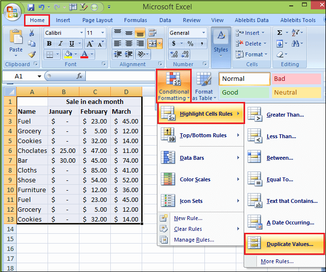
Step 4: Then, a Duplicate Values box appears. In the box next to values with, pick the formatting you want to apply to the duplicate values. 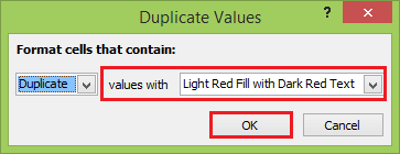
Step 5: And then click on the ok button. 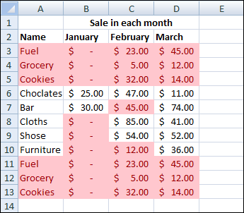
Remove Duplicate Rows using Remove Duplicate CommandRemoving duplicate value in data is a very common task. There is a dedicated command to do it in the ribbon. When you use the Remove Duplicates feature, it will permanently delete the duplicate data. Before you delete the duplicates, it's good to copy the original data to another worksheet, so you don't accidentally lose any information. Follow the following steps to remove duplicate rows by using this command. Step 1: Select a cell inside the data from which you want to remove duplicates data. Step 2: Go to the Data tab. Step 3: And click on the Remove Duplicates command button. 
Step 4: Excel will then select the entire set of data and open up the Remove Duplicates window. 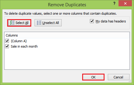
Step 5: Once you have ensured that the required fields are checked in the dialogue box, click on the ok button. 
When you press ok, Excel will remove all the duplicate values it finds and give you a summary count of how many values were removed and how many values remain. 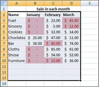
Excel deletes the duplicate rows, as required and display only the remaining unique records in the sheet. Remove Duplicates Using Advanced FilterThere is also another way to remove any duplicate values in your data from the ribbon. This is possible from the advanced filters. The Excel advanced filter has an option that allows you to filter unique records (rows of data) in a spreadsheet and copy the resulting filtered list to a new location. This gives you a data set that contains the first occurrence of a duplicated row but does not contain any further occurrences. Follow the following steps to remove duplicate rows by using the Excel Advanced Filter. Step 1: Select the data that you want to remove the duplicates. NOTE: If you select any cell within the data set, Excel will automatically select the entire data range when you activate the advanced filter.Step 2: Go to the Data tab and click on the Advanced filter Command button. 
Step 3: This will open the Advanced Filter window. 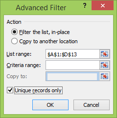
Step 4: Click on the ok button, and you will eliminate the duplicate values. 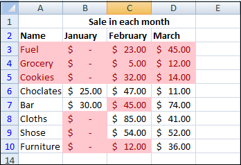
Advanced filters can be a useful option for getting rid of your duplicate values and creating a copy of your data simultaneously. But advanced filters will only be able to perform this task on the entire table. Remove Duplicate Rows Using FormulasThis method will only work if your cells' contents are less than 256 characters in length, as Excel functions cannot handle text strings that are longer than this. We will use a simple example to illustrate how to use Excel formulas to remove duplicate rows in a spreadsheet. Step 1: The first step is to combine the columns into a single column using the concatenation & operator in a new column. The formula to be entered into a new cell is: Copying this formula down all rows gives the following spreadsheet: 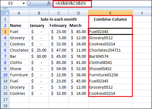
Step 2: Then highlight the rows corresponding to the duplicate values before deleting these rows. Once the contents of columns A to D have been concatenated into column E, we need to find the duplicates in the combined column E using the COUNTIF function. This function shows the number of occurrences of each value in column E, up to the current row only. 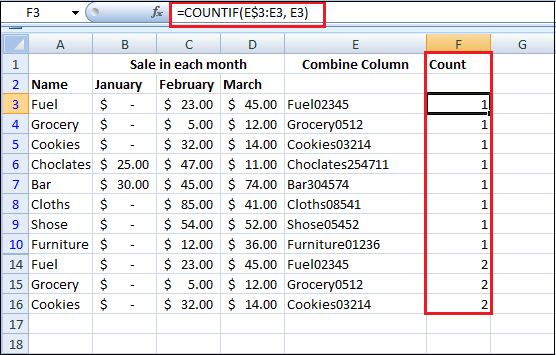
Therefore, the formula in the F3 cell returns the value 1 for the first occurrence of the text string "Fuel02345", but the formula in cell F14 returns the value 2 for the second occurrence of this text string. Step 3: Once we have used the COUNTIF function to highlight the duplicates data, we need to delete the rows for which the count is greater than 1. In the above example, it is easy to delete a single duplicate row. But, if you have several duplicates, you might find it faster to delete all duplicates at once, using the Excel Autofilter. Remove Duplicate Rows using Excel AutofilterThe following steps show how to remove several duplicate rows at once after they have been highlighted using the COUNTIF function. Step 1: Select the F column that contains the COUNTIF function in the above example. Or if you select any cell within the current data set, Excel will automatically select the entire range of data when you activate the Autofilter. Step 2: Go to the Data tab and click on your sheet's Filter button to apply the Excel Autofilter to your data. 
Step 3: Use the filter at the top of column F to select rows that are not equal to 1. Step 4: Click on the filter, and from the list of values, uncheck the value. Click on the ok button. 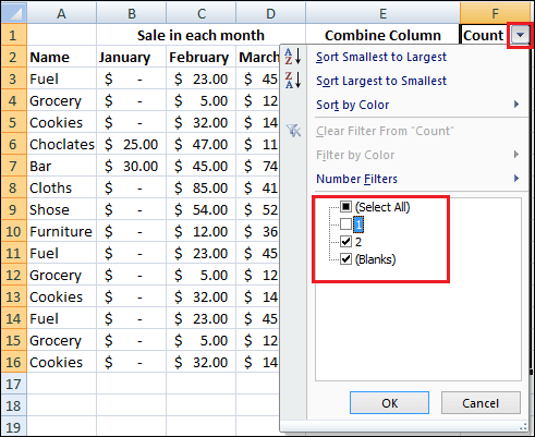
Step 5: Now, will leave with a spreadsheet in which the first occurrence of every row is hidden. And only the duplicate rows are displayed. 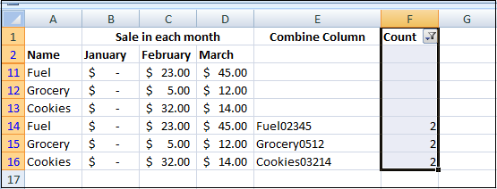
Step 6: You can delete these rows by highlighting them, then right-clicking with the mouse and selecting Delete Rows. 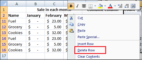
Step 7: Remove the filter, and you will leave with the spreadsheet shown below, in which the duplicate row has been removed. 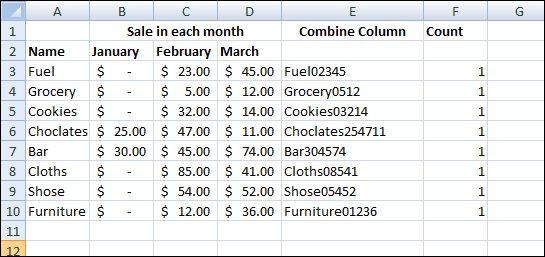
Step 8: Now, you can delete the columns containing your formulas (columns E and F in the sheet) to return to the original spreadsheet format. Remove Duplicate Rows using Pivot TablePivot tables are just for analyzing your data, but you can also use them to remove duplicate data. This method is used for both purposes, for removing duplicate values from your data or displaying only the data set's unique values. Follow the following steps to remove duplicate rows from your sheet by using the Pivot table. Step 1: Select a cell inside your data or the entire range of data. Step 2: Go to the Insert tab and click on the PivotTable button. 
Step 3: Create a pivot table based on your data. 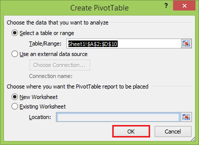
Step 4: Click on the ok button in the Create PivotTable dialogue box. 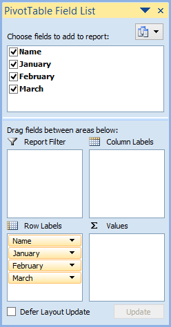
With the new blank pivot table, add all fields into the Rows area of the pivot table. Step 5: Then, you will need to change the layout of the resulting pivot table, so it's in a tabular format. Step 6: With the pivot table selected, go to the Design tab and click on the Report Layout. 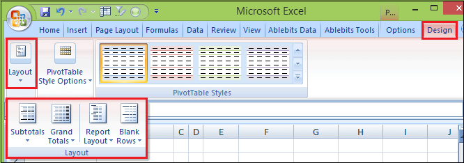
There are two options you will need to change here.
Step 7: You will also need to remove any subtotals from the pivot table. Step 8: Go to the Design tab, click on the Subtotals and then select Do Not Show Subtotals. 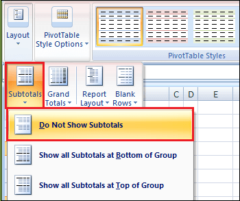
Now you have a pivot table that copies a tabular set of data. Pivot tables only list unique values for items in the Rows area, so this pivot table will automatically remove any duplicates in your data. 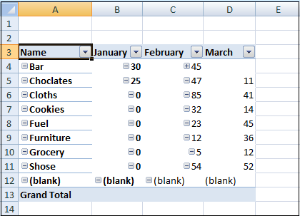
Remove Duplicate Rows Using Dedupe Table ToolUnlike the inbuilt Excel Remove Duplicate feature, the Ablebits Duplicate Remover add-in is not limited to only removing duplicate entries. This multi-tool combines all essential use cases such as identify, select, highlight, delete, copy and move unique or duplicate values, absolute duplicate rows or partially matching rows, in one table or by comparing two tables, with or without first occurrences. Assuming you have our Ultimate Excel Suite installed in your system, perform these simple steps to eliminate duplicate rows or cells: Step 1: Select any cell in the table that you want to dedupe. Step 2: Go to the Ablebits Data tab and click on the Quick Dedupe Table button. Your entire table will get selected automatically. 
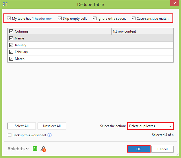
Step 3: The Dedupe Table dialogue window will be open, and all the columns will be selected by default.
As you can see, all duplicate rows except 1st occurrences are deleted. 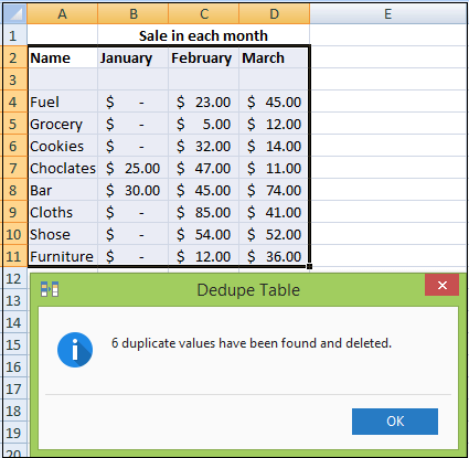
If you want to remove duplicate rows based on values in a key column, leave only that column selected and uncheck all other irrelevant columns. And if you want to perform some other action, such as highlighting duplicate rows without deleting them, or copying duplicate values to another location, select the corresponding option from the drop-down list. 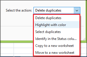
If you want more options, such as deleting duplicate rows including first occurrences or finding unique values, then use the Duplicate Remover wizard that provides all these features. Remove Duplicate Rows Using Remover WizardRemoving duplicates in Excel is a common operation. However, in each particular case, there can be several specificities. While the Dedupe table tool focuses on speed, the Duplicate Remover offers several additional options to dedupe your Excel sheets exactly the way you want. Step 1: Select any cell within the table where you want to delete duplicates. Step 2: Go to the Ablebits Data tab and click the Duplicate Remover button. 
Step 3: The Duplicate Remover wizard will run, and the entire table will get selected. The add-in will also suggest creating a backup copy, and because you are going to delete duplicates permanently, we strongly advise that you check this box. Verify that the table has been selected correctly and click on the Next button. 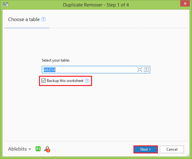
Step 4: Select what records you want to find and remove. 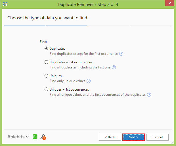
Step 5: And now, select the columns to search for duplicates. Because we aim to eliminate duplicate rows, be sure to select all the columns. 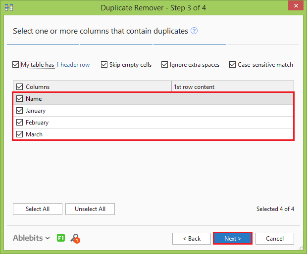
Step 6: Finally, select the action you want to perform on dupes and click the Finish button. 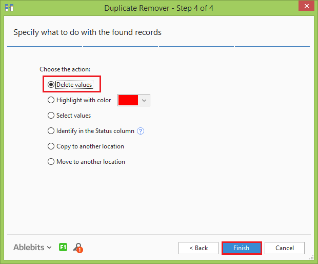
The Duplicate Remover add-in tool does its job and notifies you how many duplicate rows have been found and deleted.
Next TopicHow to use sumifs formula in Excel
|
 For Videos Join Our Youtube Channel: Join Now
Feedback
- Send your Feedback to [email protected]
Help Others, Please Share


