How to Divide and handle #DIV/0! Error in ExcelWhat is Division?"The division is a mathematical operation that involves splitting a quantity or number into equal parts or groups. It is an arithmetic operation often used to determine how often one number (the divisor) can be subtracted from another number (the dividend). The result of a division operation is called the Quotient". The division operation is represented by the symbol � or /; the numbers involved are the dividend, divisor, and Quotient. The dividend is the number divided, while the divisor is the number divided. The Quotient is the result of the division operation. For example, if we divide 12 by 3, we can say that we are splitting 12 into three equal parts. The Quotient, in this case, is 4, which means that 12 can be divided into three parts, each equal to 4. We can represent this division operation as 12 � 3 = 4, or 12/3 = 4. It is important to note that Division by zero is undefined, as splitting a quantity into zero parts is impossible. Purpose of Division in ExcelThe purpose of Division in Excel is to perform mathematical calculations that involve dividing one value by another. This can be useful in many contexts, such as financial analysis, scientific research, or statistical calculations. Some common examples of how Division can be used in Excel include:
Methods to divide the values in ExcelExcel provides various functions and formulas to perform Division in Excel. The methods are explained as follows, 1. Using the "/" operatorIn Microsoft Excel, Division is a mathematical operation that can be performed using the "/" operator. To use the "/" operator for Division, enter the divisor after the dividend in a cell. Excel will then perform the division operation and display the result in the new cell. For example, to divide the value present in cell A1 by B1, enter the formula in a new cell as A1/B1. 2. Quotient functionThe syntax of the QUOTIENT function is: Where, "numerator" is the dividend or the number being divided, and "denominator" is the divisor or the number doing the dividing. For example, if you want to find the Quotient of 13 divided by 4 using the QUOTIENT function, you would enter "=QUOTIENT (13, 4)" in a cell. The function will then return the value 3, the integer quotient resulting from dividing 13 by 4. It is important to note that the QUOTIENT function always rounds down to the nearest integer. If you need to round the result of the division operation to a specific number of decimal places, you should use the ROUND function in conjunction with the QUOTIENT function. 3. MOD FunctionThe MOD function in Excel is a mathematical function that returns the Remainder of a division operation. It calculates the modulus of two numbers, the amount by which one number is greater than the largest multiple of the other number that is less than it. The syntax of the MOD function is as follows: Where, "number" is the dividend or the number being divided, and "divisor" is the divisor or the number doing the dividing. The MOD function can be useful in various contexts, such as determining if a number is even or odd, calculating periodic payments, or working with clock or calendar calculations. How to perform Division in ExcelTo perform Division in Excel, some of the examples are explained here. The steps to be followed are, Example 1: Divide the values present in column A by column B.
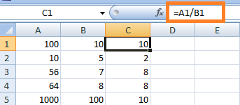
Example 2: Divide the given values by the specified divisor. In this example, the given value is divided by the user-defined divisor. The steps to be followed are,
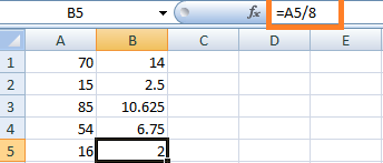
Example 3: Divide column A into column B using the Array formula An array formula in Division is a formula that performs a division operation on a range of cells instead of just two cells. It allows you to divide the values into multiple cells by the values in corresponding cells in another range, all at once. To create an array formula in Division, you need to follow these steps: Step 1: Select the range of cells that you want to divide by another range of cells. Here the range of cells is present in A1:B5. Step 2: Type the division symbol ("/") followed by the range of cells you want to divide by, enclosed in parentheses. To divide each of them by the corresponding range of numbers, you can create an array formula in cell C1 with the following formula: = A1:A5 / (B1:B5) Step 3: Instead of pressing Enter, press Ctrl+Shift+Enter. This will divide each number in the range A1:A5 by the corresponding number in the range B1:B5 and return an array of results in the same shape as the original ranges. 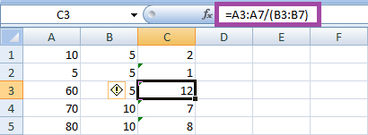
How to get the Quotient of the dividing values?As previously explained, the Quotient function is used to get the Quotient of the dividing values. The steps to be followed are, Step 1: Enter the data in the worksheet respectively, namely A1:B5 Step 2: Select a new cell where the user wants to display the result, namely C1, and enter the formula as =Quotient (A1, B1) Step 3: Press Enter. The Quotient will be displayed in cell C1. To get the result for the remaining cell, drag the Fill handle toward cell C5. 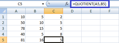
How to get the Remainder of the dividing values?As previously explained, the Remainder function gets the Remainder of the dividing values. The steps to be followed are, Step 1: Enter the data in the worksheet respectively, namely A1:B5 Step 2: Select a new cell where the user wants to display the result, namely C1, and enter the formula as =MOD (A1, B1) Step 3: Press Enter. The Remainder will be displayed in cell C1. To get the result for the remaining cell, drag the Fill handle toward cell C5. 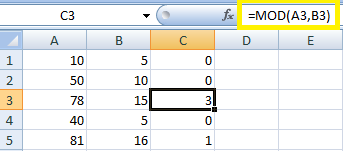
How to divide by Percentage in Excel?To divide a percentage in Excel, you can divide the percentage value by 100 or by another number. Here are the steps: Step 1: Enter the percentage value you want to divide into a cell, A1, as 100. Step 2: Enter the divisor value into another cell, B1, as 50. This can be a constant number or a reference to another cell containing the divisor value. Step 3: Enter the division formula using the "/" operator in a third cell. For example, if your percentage value is in cell A1 and your divisor value is in cell B1, you can enter the formula "=A1/B1" into cell C1. 
Step 4: To display the result as a percentage, you can format the cell as a percentage. To do this, select the cell with the result, right-click, and choose "Format Cells." In the Format Cells dialogue box, select "Percentage" under the "Category" list, and choose the desired number of decimal places. 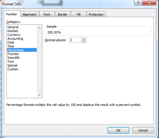

Alternatively, you can use the formula "=A1% / B1" to divide a percentage value by another number. This formula divides the percentage value by 100 and then divides the result by the divisor value. This can be useful if you want to divide a percentage value already formatted as a percentage. Divide the values present in the Column using Paste Special OptionThe "Paste Special" option in Excel allows you to paste the clipboard's content in various formats or perform calculations on the data you're pasting. In this example, the data in single columns are divided by the same number. The steps to be followed are, Step 1: Enter the data in the worksheet, namely A1:A5 Step 2: Copy and paste the values present in Column A1:A5 to Column B1:B5 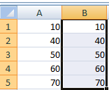
Step 3: Enter the divisor value in the new cell, D1. Step 4: Copy and paste the divisor value in the new cell, namely D4. 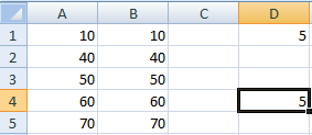
Step 5: Select the range of cells which needs to divide, namely B1:B5. Step 6: Press Ctrl+Alt+V, and the Paste Special dialogue box will appear. Choose the option "Divide." Click Ok. 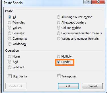
The Paste Special option divides the values in Column B1:B5 with the divisor value. 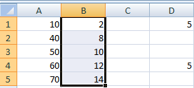
Dividing a Single column of values with Absolute and Relative referenceFrom the above method, the formula we used to divide a column of numbers is =A1/Specified Number. Here Specified Number is called a relative reference. In Excel, a relative cell reference refers to a cell or range of cells based on its position relative to the cell containing the formula. For example, if you have a formula in cell B2 that refers to cell A2, the reference to A2 is relative because it is based on its position relative to the formula in B2. If you copy the formula from B2 to cell C2, the reference to A2 will change to B2 because it is now based on its position relative to the new formula in C2. Relative cell references are useful when you want to copy a formula to multiple cells and have it update automatically based on its new position. This can save time and prevent errors, as you don't need to update each reference in the formula manually. To indicate a relative reference in Excel, reference the cell or range of cells using their column and row labels. For example, the relative reference for the cell to the left of the current cell is "A1". Step 1: Enter the data in the worksheet, namely A1:A5 Step 2: Select a new cell, B1, and enter the formula as =A1/5. Step 3: To display the result for the remaining data, drag the fill handle toward cell B5. 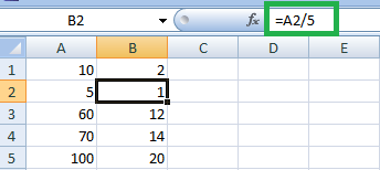
In this example, the formula gets suited according to each row as in B2, and the formula becomes A2/5. For B3, the formula becomes A3/5. For B4, the formula becomes A4/5. For B5, the formula becomes A5/5. Divide using Absolute ReferenceIn Excel, an absolute cell reference refers to a specific cell or range of cells that do not change when the formula is copied to other cells. This contrasts a relative cell reference, which changes based on its position relative to the cell containing the formula. Absolute cell references are useful when referring to a fixed cell or range of cells in a formula. For example, if you have a formula that multiplies a value in cell A1 by a fixed value in cell B1, you would want to use an absolute reference for cell B1 so that it does not change when you copy the formula to other cells. To create an absolute reference in Excel, use the dollar sign ($) before the column letter and row number in the cell reference. For example, the absolute reference for cell B1 would be $B$1. When you copy the formula that contains an absolute reference to other cells, the reference to $B$1 will not change. In contrast, the relative references will change to reflect their new position relative to the formula. Step 1: Enter the data in the worksheet, namely A1:A5 Step 2: Select a new cell, B1, and enter the dividend value. Here the dividend value is entered as 5. Step 3: In cell C1, enter the formula as =A1/$B$1. Press Enter. Step 4: The result will be displayed in cell C1. To display the result for the remaining data, drag the fill handle toward cell B5. 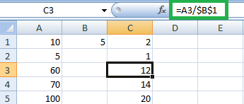
In the worksheet, the divisor is entered in the new cell and referred to using absolute reference in the formula. What are the common errors that occur while dividing the values in Excel?There are a few common errors that can occur when dividing in Excel. Here are some of the most common ones:
How to handle #DIV/0! Error in Excel?The #DIV/0! error in Excel occurs when a formula attempts to divide a number by zero or an empty cell. Here are some ways to handle this error: 1. Use the IFERROR function The IFERROR function replaces the error value with a custom message or a blank cell. For example, =IFERROR (A1/B1, "N/A") will display "N/A" instead of the #DIV/0! error when A1/B1 results in a division by zero error. Step 1: Enter the data in the worksheet, namely A1:B5 Step 2: Select a new cell, namely C1, where the user wants to display the result and enter the formula as =A1/B1. Step 3: Press Enter. The result will be displayed in column C1. Drag the fill handle towards column C5 to display the result for the remaining data. 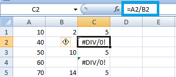
Here is worksheet #DIV/0! The error occurs. To handle this error, replace the formula with =IFERROR (A1/B1,"). The result will be displayed as shown, 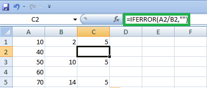
2. Use the IF function Another option is to use the IF function to check for a zero or empty cell before performing the Division Division. For example, =IF (B1=0, "N/A", A1/B1) will display "N/A" if B1 is zero and perform the division if B1 is non-zero. Step 1: Enter the data in the worksheet, namely A1:B5 Step 2: Select a new cell, namely C1, where the user wants to display the result and enter the formula as =IF (B1=0,", A1/B1), or the formula can be written as =IF (B1<>0, A1/B1,"). Instead of displaying empty cells, to display the error message, one can modify the formula as ==IF (B1<>0, A1/B1, "Error in Calculation") Step 3: Press Enter. The result will be displayed in column C1. Drag the fill handle towards column C5 to display the result for the remaining data. 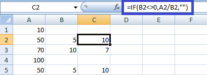
3. Use a conditional formatting You can also use a conditional format to change the appearance of cells that contain the #DIV/0! Error. For example, you can apply a red background color to cells that contain the error to make them stand out. 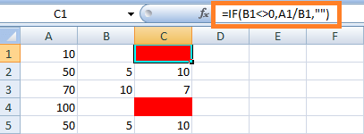
Check for data input errors: If you see the #DIV/0! Error frequently in your spreadsheet. It may be worth checking for data input errors, such as missing or incorrect values, causing the error. SummaryIn conclusion, Division is a basic arithmetic operation in Excel that allows you to calculate the Quotient of one number divided by another. The division operation is performed using the forward-slash (/) operator, and you can use either constant values or cell references in your division formula. Excel will automatically calculate and display the result of the division operation in the cell where you entered the formula. The division is a fundamental Excel tool used in many calculations, such as percentages, ratios, and averages. |
 For Videos Join Our Youtube Channel: Join Now
Feedback
- Send your Feedback to [email protected]
Help Others, Please Share


