| |

How to compare two columns in Microsoft Excel for matches and differencesIt was well known that making comparisons of the particular amounts of the columns in Microsoft Excel is something unique which can be done or performed in one sort of action very well. Microsoft Excel offers different options to make comparisons of the data as well as the matching of the data accordingly. On moving ahead, in this tutorial, we will be exploring and discussing the various techniques that can be used to compare two columns in Microsoft Excel. We can also find matches and the differences between them efficiently.
How can we compare two columns in Microsoft Excel row by row?When we are moving on performing a data analysis in Microsoft Excel, in that case one of the most valuable tasks is efficiently comparing of the data in every particular row. And this task can be very well achieved or done with the help of the IF FUNCTION as it was depicted in the below-discussed formula. # Method 1: Comparisons of two columns for doing matches or differences in the same rowIn these examples, if we need to compare two respective columns in Microsoft Excel row by row, then we will be writing out a usual formula that is none other than the IF formula, which is used to compare the first two cells. After that, we will be then moving further by entering the formula in some other column within the same row, and then after we will copy it down to other cells and this could be achieved by just dragging the fill handle. And when we perform this, then the cursor will get changes to the plus sign respectively. 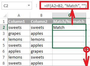
The formula which can be used for the finding of the matches in Microsoft Excel Now to find the individual cells within the same row that in turn have the same content, A2 and B2 in this example and the formula that can be applied to it is as follows: A formula which can be used for finding the differences in Excel Now for the purpose of finding out the cells for the same row which are having the different values, then in that case we can easily replace the equals sign via the non-equality movement (<>). Matches and differences in Microsoft Excel Moreover, in Excel it was well known that there is nothing which can prevent us from finding the differences and the matches with the help of a single formula respectively. Or And the result of outcomes of the above will look much similar to this: 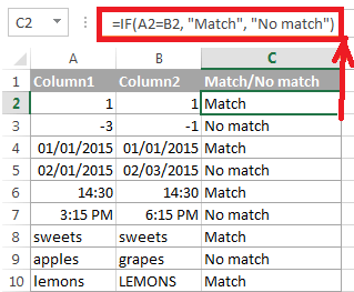
We have seen that the formula primarily handles the dates, numbers and strings equally well. Important point: It was well known that we can also compare the two columns row by row with the help of the Microsoft Excel Advanced Filter. Here is an example depicting how we can filter the matches and the difference between the 2 columns. # Method 2: Making comparisons of the two lists for case-sensitive matches in the same rowWe all know that the formula which we have used previously ignore the case whenever we are making comparisons of the text values as it was seen in the row 10 as well. And if in case we need to find out the case-sensitive matches existing between the 2 columns in each row, we can make use of the EXACT function as mentioned below: 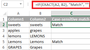
Making comparisons of the multiple columns for matches in the same rowSo in these we will be able to see with the help of the example that how we can make comparisons of the multiple columns for matches in the same respective row: # Example 1: Finding out the matches in all cells within the same row In these case our particular table which is consisting of three or more columns and we need to figure out all the rows that are consisting of the same values in all the cells, so in that scenario we can make use of the IF formula with an AND statement: 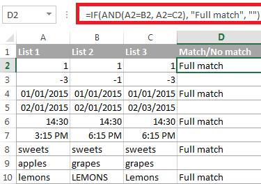
And if in case our selected table has got lots of columns, then we would be using the function COUNTIF: =IF (COUNTIF ($A2:$E2, $A2) =5, "Full match", "") And in these, 5 is the number or value representing the number of the columns we are comparing out efficiently. How we can make comparisons of two given columns for matches and finding the differences in Microsoft Excel?And to understand these very easily, we will be taking out the 2 lists of the data in Microsoft Excel, and then we are supposed to figure out or find all the values which are there in column A but not in column B. Moreover to achieve this, we can combine the COUNTIF ($B:$B, $A2)=0 functions in IF's logical test and then can perform checks if it returns zero value, then we can say that no match has been found and vice-versa. After that the following IF or the COUNTIF formula moves on searching all across the entire column B for the value in cell A2. And if no match is found then we will get an output that "No valid match exists." 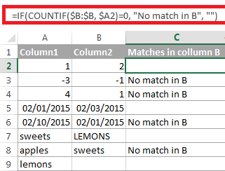
Points to be noted: It was known that our table has a fixed number of rows, which we can specify a specific range (e.g. $B2:$B10) instead of using the entire column ($B: $B) for the respective formula in order to work much faster on the huge sets of the data which are available to us. Moreover, the same result or the outcomes can be efficiently achieved with the help of the IF formula with the embedded ISERROR as well as the MATCH functions, which are primarily available in Microsoft Excel: Comparing the two lists as well as highlighting matches as well as the differencesIn many case, we may need to "visualize" the items primarily present in one of the columns, but they could also be missing in the other column. Furthermore, we can shade such respective cells in any particular color of our choice with the help of the Excel Conditional Formatting feature and the following examples, which are depicted below with the detailing of the step. # Example 1: Ensure the highlighting of matches and the differences in each row in excel For making comparisons of the two columns as well as highlighting the cells from the given column that is Column A which have identical entries in the given column B in the same row, we will perform the steps which are as follows: Step 1: First of all, we will be selecting out the particular cells which we want to highlight it. Step 2: After that, we will click on the Conditional formatting > New Rule? > and then click on Use a formula to determine which cells need to be formatted. Step 3: And now, in this step, we will create a rule with the help of the simple formula such as =$B2=$. 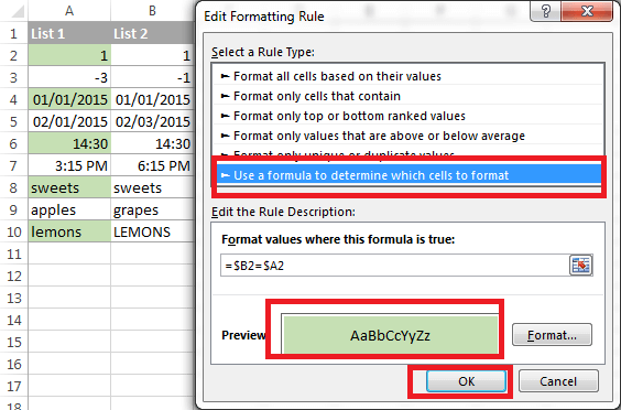
And if in case we need to highlight the differences between columns A and B, we can create a rule with the help of this formula as well: 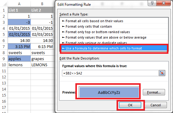
# Example 2: Highlighting the unique entries in each list of the excel sheet And when we are making the comparison of the two lists in Microsoft Excel, there exist 2 item types which we can highlight: The Items which are only in the 1st list (unique) The Items which are only on the 2nd list (unique) Now in this example, we will demonstrate how to color the items which are there in one list respectively. For this we are having the List which are present in the different column such as: List 1 is in column A (A2:A6) as well as List 2 is in column C (C2:C5). And we need to create the conditional formatting rules with the help of the following formulas: Highlighting of the unique values which are present in 1 (column A): Highlighting of the unique values which are present in the List 2 (column C): We will get the following output respectively: 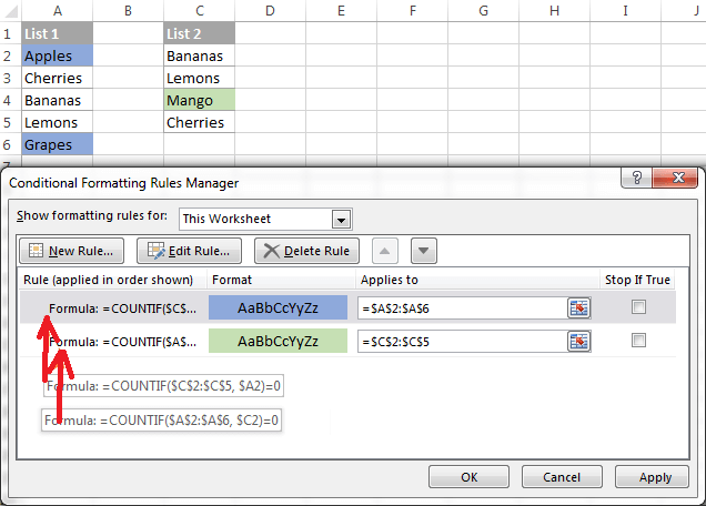
|
 For Videos Join Our Youtube Channel: Join Now
Feedback
- Send your Feedback to [email protected]
Help Others, Please Share


