How to Prevent Text Spilling in Excel?

What is called Text Spilling?

Data entered by the user in the spreadsheet sometimes exceeds the cell which causes spilling over the adjacent columns. In Microsoft Excel, Text spilling refers to the overflow of Text from a cell into adjacent cells when the Text in the original cell exceeds the width of the column or the row's height. This can occur when the cell needs to be wider to display all of the Text or when the Text is too long to fit within the row's height.

Causes of Text Spilling

There are several reasons for Text spilling in Excel. The reasons are listed below as follows,

1. Column Width is too narrow: When the width of a column is not wide enough to display the Text in a cell, the Text will spill over into adjacent cells.
2. Row height is too short: When the height of a row is not tall enough to display the Text in a cell, the Text will spill over into adjacent cells.
3. Text wrapping is turned off: By default, Text in Excel cells is not wrapped. If text wrapping is turned off and the Text in a cell is too long to fit within the cell's boundaries, the Text will spill over into adjacent cells.
4. Cells are merged: When multiple cells are merged into one cell, the Text in that cell can spill over into adjacent cells if the merged cell is not wide enough or tall enough to display all of the Text.
5. Text overflow from a formula: If a formula in a cell produces Text that is too long to fit within the cell's boundaries, the Text will spill over into adjacent cells.

Methods to Prevent Text Spilling in Excel

Excel provides various methods to prevent Text from spilling into adjacent cells. The methods are explained as follows,

1. Alignment Option

The Alignment option in the Excel home tab prevents the Text from spilling in Cells. The steps to be followed are,

Step 1: Enter the data in the worksheet, namely A1:A5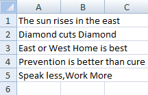

Step 2: Here, the data present in cell A1:A5 exceeds its cell and spills into adjacent cells. Select the cells to prevent spilling. The cell range A1:A5 is selected.

Step 3: Click the Dialog launcher in the Alignment group in the Home Tab.

Step 4: The Format Cells dialog box will open. In that, click the alignment group. Choose the option "Fill" from the drop-down list in the Horizontal tab.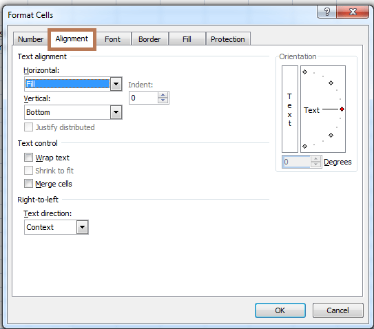

Step 5: Click Ok. The data present in cell range A1:A5 are truncated within the cell boundary.

Note: If all the data in the selected range is spilled, this method truncates the data. For example, in the selected cell range, if a cell contains data that is already cropped like, "hi," the result will be "hi hi hi." The Fill option will populate the entire content in a repeated manner.

2. Wrap Text

Wrap Text is a feature in Microsoft Excel that allows Text to automatically wrap within a cell to fit within the cell's boundaries. When wrap text is enabled, the Text in a cell will automatically adjust to fit within the column width, even if the Text is too long to fit in one line.

The steps to be followed to use Wrap text are as follows,

Step1: Enter the data in the worksheet, namely A1:A5

Step 2: Here, the data present in cell A1:A5 exceeds its cell and spills into adjacent cells. Select the cells to prevent spilling. The cell range A1:A5 is selected.

Step 3: Choose the Wrap text option from the Alignment group in the Home tab.

Step 4: The selected Text will be wrapped as follows,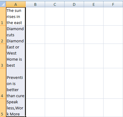

To display the row height the same as before, the steps to be followed are,

Step 1: Before applying the wrapping text function, click the Format>Row Height option. It displays the current row height. By default, it displays the row height as 15. The point may vary depending on the font size in the worksheet.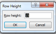

Step 2: Click Ok. Now apply the wrap function to the selected data. The row height remains the same.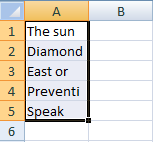

3. Using the Space bar and the Ctrl+Enter option

Here Excel provides another method using a shortcut to prevent spilling the data. The steps to be followed are,

Step 1: Enter the data in the cell range, namely A1:A5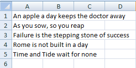

Step 2: Select the adjacent cell range to the overflowing cell range. Here the cell range B1:B5 is selected, as A1:A5 is called the overflowing cell range.

Step 3: After selecting the adjacent cell range, press Spacebar.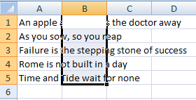

Step 4: Without disturbing the selection, press Ctrl+Enter. The function inserts the space in each of the selected cell ranges.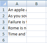

The worksheet's adjacent columns (B1:B5) look empty, but no text flows into them from the left.

Sometimes the columns contain a combination of shorter and longer Text where the longer Text overflows to the adjacent cell. Hence this makes the data to be in a different form. To display the data in an even form, a similar method called Method 3 is implemented.

Example: In this worksheet, the data overflow to the adjacent columns. Prevent data spilling using the shortcut.

Step 1: Enter the data in the worksheet, namely A1:A5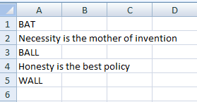

Step 2: Here, cells A2 and A5 spill the data, as the remaining data fit the cell. Select the adjacent column next to the spilling data to make all the data even.

Step 3: Here, the cell range B1:B5 is selected, and choose the option Find & Select in the Edit group in the Home tab.

Step 4: In the Find & Select option, select "Go to Special" or Press F5.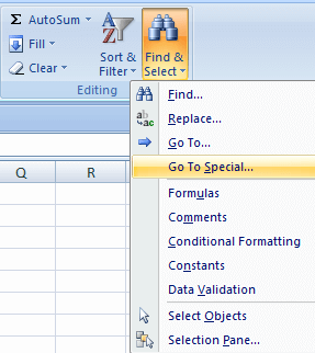

Step 5: The Go to Special dialog box will appear. In that choose the option "Blanks." Click Ok.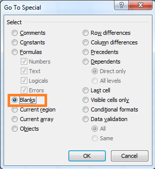

Step 6: With the blank cell selected, type Spacebar and press Ctrl+Enter. Now the adjacent columns' cell range is inserted with blank cells.

Note: In this method, no data is spilling into the next columns, but the data of the overlapping cell needs to be fully seen if it is selected. Hence based on the data requirement, the method needs to be chosen.

Summary

In Microsoft Excel, Text spilling is a common issue that can be easily resolved using one of the methods above.