#N/A error in Excel

Encountering an Error is normal, but later on, fixing those errors is what makes you an Excel in Excel. There are different reasons why one experiences error values in the Excel worksheet. However, there are several types of error values like #DIV/0, #NAME?, #NULL!, #NUM!, #REF!, #N/A, and #VALUE! But today, we will cover the #N/A error value. There are a few fundamental reasons why the VLookup #N/A error is generated in the Excel sheet.

In most cases, the #NA! error occurs if something went wrong with the lookup tables, it could also pop up if mistakenly the user has skipped an important element in their formula. If you're facing #N/A errors on your Excel worksheet, don't worry; in this tutorial, we will show you the various steps to trace and fix this error. But before we move any further, let's conclude the definition of #N/A! Error.

What is #N/A error in Excel?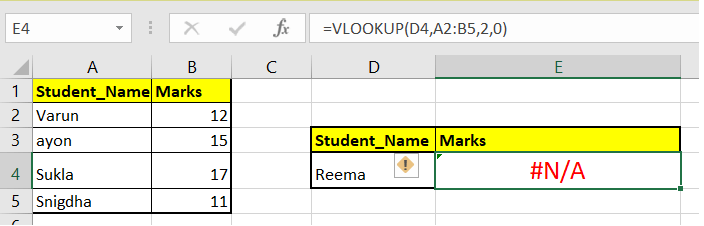

"The #N/A error appears whenever the value can't be found or identified in your Excel worksheet. It generally occurs in formulas unlike classic lookup functions, i.e., VLOOKUP, HLOOKUP, LOOKUP and MATCH, when Excel couldn't locate the exact value from the referenced data. However, the #N/A error can also be found if the user has used extra space characters or misspellings."

The #N/A error is commonly related with lookup tables, but it is most likely to occurs because of one of the following reasons:

1. You've entered some data in your formula that Excel can't locate.
2. If you forget to insert a significant element in your Excel formula.

This error is considered a useful error, because it informs the user that something is missing- an element is not used, values are misspelled or required colon option is not give, etc.

Sometimes we intentionally have to use empty cells since we are not given the values for the respective field. For such cases, we can use NA to mark the empty cells. By typing N/A in cells for missing data, you can bypass the problem of mistakenly including the empty cells in your calculations.

NOTE: If your formula refers to a cell containing the #N/A, it will return the #N/A error value.

How to Fix #N/A error in Excel?

In the above section of this tutorial, we learnt about the #N/A error and the various situations where Excel can throw the #N/A error. However, there are various methods using which we can get rid of this error. Now let's look at the multiple tricks to fix this error in excel:

• Check whether there any extra characters (for instance space characters).
• Check whether any required data has been missed.
• Whether the lookup table has some additional or unwanted data.

The quick way to get rid of the #N/A errors is to make sure values and tables used are in your Lookup formula are correct and complete. If that's accurate in your case, below are few extended measures that you can check to prevent this error:

1. Whether the lookup value in your Excel worksheet is spelled correctly and make sure it does not contain any extra space characters.
2. Your lookup table should contain all the required values.
3. Check whether the specified lookup range mentioned in the function is complete or not.
4. The specified lookup value type should match the lookup table type (i.e., both should either be text or numbers, etc.)
5. The matching (approximate vs. exact) of the formula should set correctly.
6. Verify whether in the lookup formula the range entered is complete or not.
7. Check if the type of lookup value and lookup table match. Both should either be text strings, numeric values, etc.

How to Fix #N/A error?

Errors can also be fixed using a Excel functions such as:

• IFERROR
• IFNA

#1 - Using the IFERROR Function to fix the error

The Excel IFERROR function helps to rectify and tackle the #N/A error. This function returns an alternative output instead of the Error output, making your worksheet look more professional.
For example, we know if we apply an AVERAGE formula to string values, it will return an error since Average is a numerical formula and cannot be if we find the Average of String data types, it will throw an error.

If you are sharing business data with others, in such cases, the occurrence of errors makes your sheet look unprofessional. In such cases, an alternative statement would be the best solution. Therefore, we can apply the IFERROR function to fetch an alternative output of "There are some issues, kindly check the formula again" whenever our Excel worksheet throws a #N/A Error.

Below given is the VLOOKUP formula that we have implied in our worksheet:

=VLOOKUP(D5,A2:B6,2,0)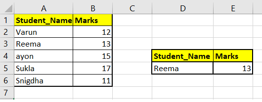

Initially, when you write and verify the formula, everything works well. With time, you do some activity. Let's suppose you deleted a value of a cell that was directly included in our formula. Since Reema's entry has been deleted from the table, Excel can't find any such value in the VLOOKUP and throw the N/A error.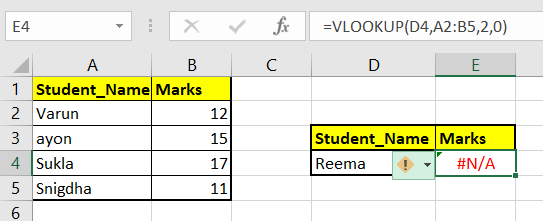

Well, to avoid the random occurrence of N/A error, the best solution is to trap the error with the help of the IFERROR function, Following are the steps to trap an error using IFERROR:

1. Start the formula with '=' ( equals to) followed by the IFERROR.

2. In the value argument, we will specify the Vlookup formula

3. In the value_if_error formula, we will type the alternative text you want the formula to return in case the #N/A error is trapped.

=IFERROR(VLOOKUP(D4,A2:B5,2,0), "Something went wrong, recheck the formula!")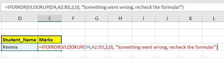

4. Press enter to run the formula. You will have the following output.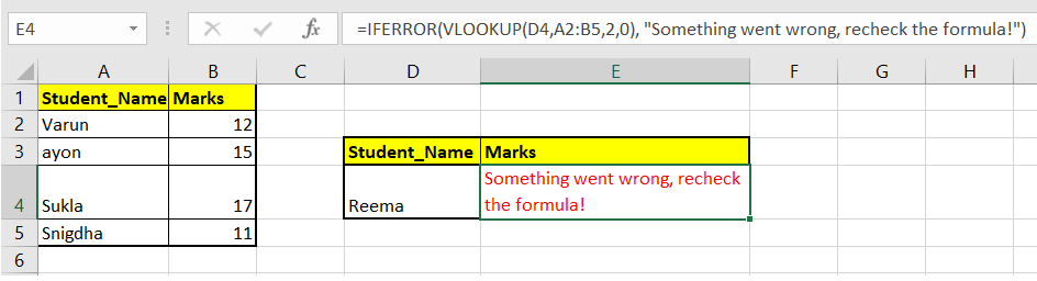

As a result, you will notice that the IFERROR has returned the alternative text value.

Note: The above formula is not limited to #N/A error. It can trap any Excel error.

2. Fixing the #N/A Error Using the IFNA Function

Misspelling a function name is quite common in Excel, and we all face this problem a day or other while working with worksheets. Whenever it happens, you might have noticed that Excel returns the #NAME? error. However, if you apply the IFERROR function, it acts as a blanket solution. Therefore, you won't get to know whether the error is a #N/A error or #NAME? error because IFERROR is a standard function that traps all errors.

Fortunately, there's a solution for this. If you only want to catch the #N/A errors, instead of IFERROR, try the IFNA function. The IFNA function mainly detects the #N/A errors. If your formula returns any other error, in such cases, Excel won't replace the alternative output and will throw the error.

Applying the IFNA function is helpful if you only want to target the #N/Averror. For example, in the above table you see Sukla score still exists because of a misspelt VLOOPUP formula the IFERROR function is returning the substitute output.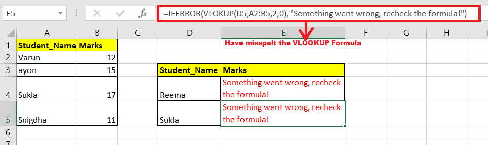

In the case of the IFNA function, it will screen out the alternative output. Following are the steps to trap a #N/A error using IFNA:

1. Start the formula with '=' ( equals to) followed by the IFNA.

2. In the value argument, we will specify the Vlookup formula

3. In the value_if_error formula, we will type the alternative text you want the formula to return in case the #N/A error is trapped.

=IFNA (VLOOKUP(D5,$A$2:$B$6,2,0), "Player Not Found")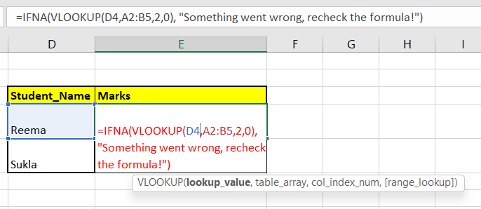

4. Press enter to run the formula. You will have the following output.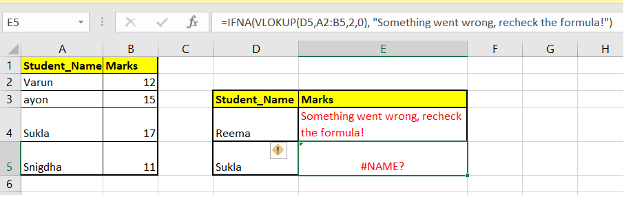

As a result, you will notice that the IFNA has returned the alternative text value because the VLOOKUP resulted in a #N/A error. For the second field, it ends up returning the #NAME? error because it only traps #N/A error.

3. Force #N/A Error

So far, we have covered various functions using which we can substitute the #N/A error with some other customised values. But did you know that Excel has also introduced the NA function that forces the formula to return the #N/A error in case any value goes missing from your worksheet, and later, using the IFNA function, you can trap the error.

What is NA() function?

The NA() function was introduced to mark the empty cells. This function returns the error value #N/A.

Syntax

Parameters

The NA function syntax has no parameter.

Ideally, this function is used whenever the user wants to throw the #N/A error. For example, for every negative value if you want to return the #N/A error, you can merge the NA function with IF conditional and construct your formula. You can use the following formula:

=IF(A1<0,NA(),A1)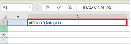

As a result, the formula will return the #N/A error if cell A1 contains any negative number. If the referenced cell has positive number, it will return the number itself.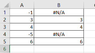

You can further edit the formula and trap the error using the IFNA function and can return your customised message. You can use the following formula:

=IFNA(IF(A1<0,NA(),A1), "You have entered a negative number")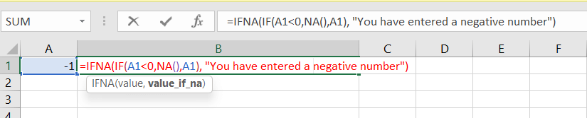

That's all! We have covered almost everything you need to know about #N/A error in this tutorial. So next you end up having #N/A error; you can quickly get rid of it!