| |

Excel IFNA FunctionIf you are an Excel user, you may know how annoying and time-consuming the errors could be. Most of the time, when you work with functions unlike HLOOKUP, VLOOKUP, MATCH, etc., you encounter the #N/A error. The blunt #N/A looks unprofessional and messy when you present the formula sheet to your colleagues or the management. Now the question arises of how to deal with this error. To your, surprise Excel has provided a solution for this as well. You can use the inbuilt IFNA Excel function to replace the #N/A error with your customized message. What is IFNA function?The Excel IFNA function is introduced by Microsoft to specifically trap and manage #N/A errors in your worksheet, ignoring the other errors. This function returns the customized message that you have specified if Excel finds any #N/A error value in the function; else, in case of no error, IFNA returns the result of the formula. Instead of using the IFERROR function (that traps all types of errors), you can switch to the IFNA function to catch and handle #N/A errors specifically that may appear in functions that execute lookup formulas such as MATCH, VLOOKUP, HLOOKUP, etc. The IFNA function returns a customized output whenever Excel traps any #N/A, and the good part is that it returns normal output if no error is detected in your worksheet. Please note that the IFNA function will only handle #N/A errors, and all the other Excel errors will still be displayed in your Excel sheet. The IFNA function falls under the category of Excel Logical functions. NOTE: Microsoft Excel has introduced the IFNA function in Excel 2013 version, so if you are working with an older version of Excel, you may not find this function.Syntax Parameters
ReturnThe IFNA function returns a customized output whenever Excel traps any #N/A, and the good part is that it returns normal output if no error is detected in your worksheet. Points to Remember for IFNA function
ExamplesExample 1: Divide Col A by Col B and show the results using IFNA function.IFNA becomes very useful when you only want to catch only the #N/A error. To trap and handle #N/A errors using the IFNA function follow the below-given steps: STEP 1: Add a helper column named "Output using IFNA"Place your mouse cursor to the cell next to "ColA" and name the new column as "Output using IFNA". It will look similar to the below image: 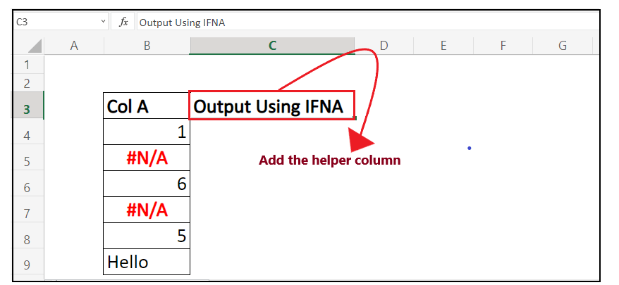
In this column we will type our IFNA formula and will trap #N/A errors for different data values. NOTE: Format the helper column and match it with the first column to make your Excel sheet more attractive.STEP 2: Type the IFNA formulaPut your cursor to the second row and start typing the function = IFNA( It will look similar to the below image: 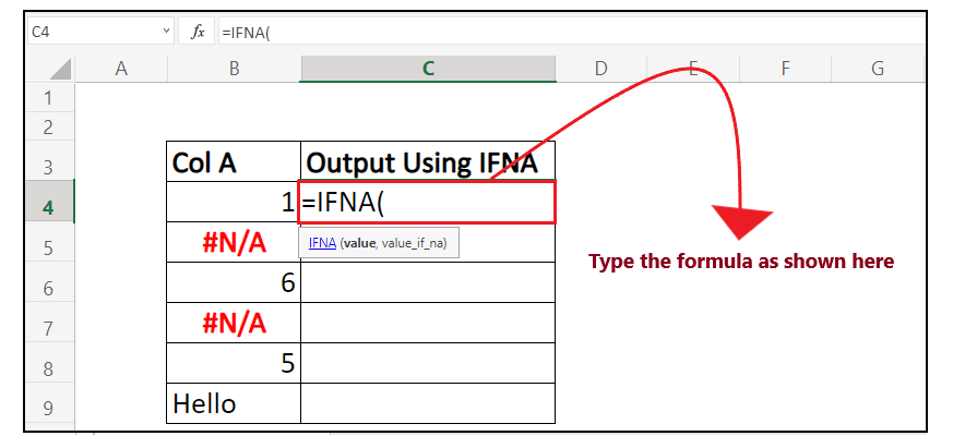
STEP 3: Insert the text parameter
It will look similar to the below image: 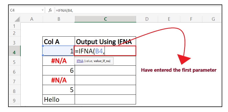
It will look similar to the below image: 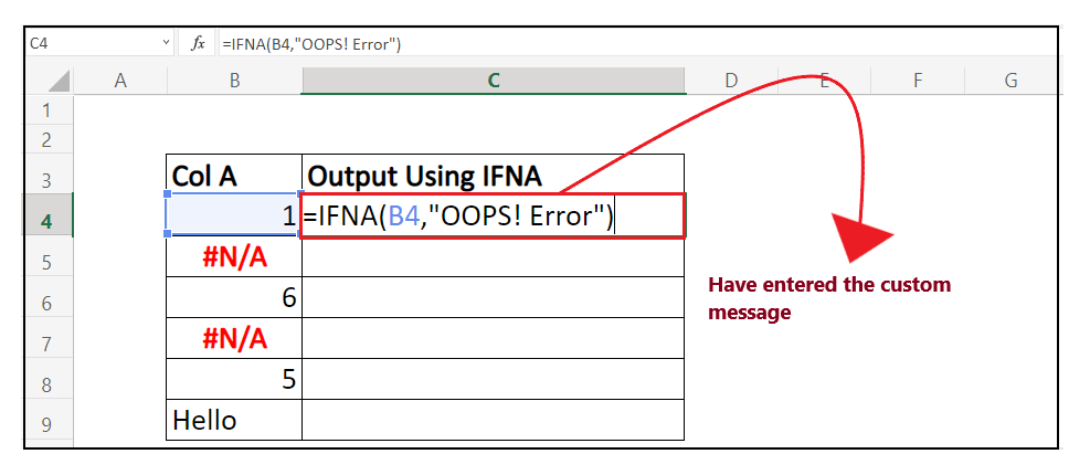
STEP 4: IFNA will return the resultSince IFNA has found no #N/A error, so it has returned the original value. When we apply the formula for the next row, we will see what happens if it encounters a #N/A error. It will look similar to the below image: 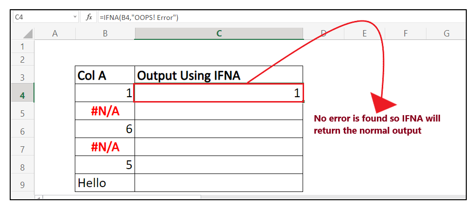
STEP 5: Drag the formula to other rows to repeatPlace your mouse cursor on the formula cell and point the cursor to the right corner of the cell. To your surprise, the mouse pointer will turn into a '+' icon. Refer to the below image: 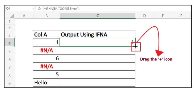
Drag the '+' icon down the cells. It will copy the function to all your cells, changing the cell reference as respective to the cell. As you can see below, when the function encounters #N/A error, it is handled by the IFNA function, and it replaces "#N/A" with the custom text "OOPS! Error" and displays it. It will look similar to the below image: 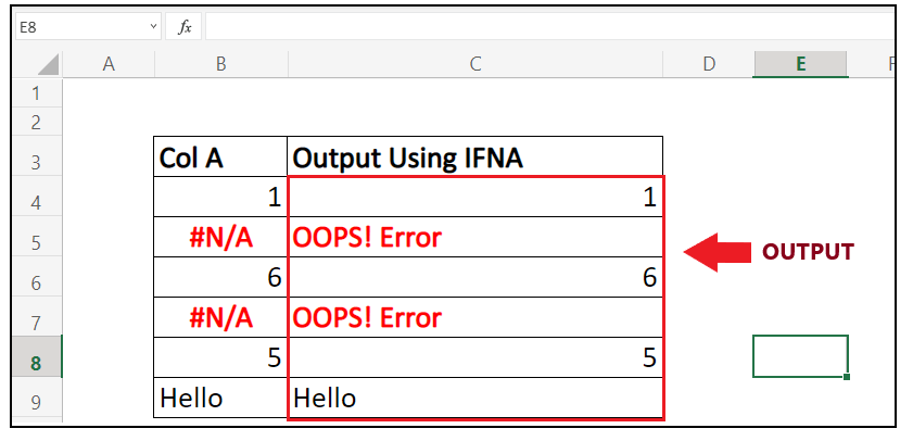
That's it; following the above few steps, you easily apply the IFNA function to your Excel worksheet to handle the # N/A errors. Example 2: Using the IFNA function find the monthly salary of the given employees and if #N/A appears, then change it to ERROR IN SALARY.
IFNA function becomes handy when you are dealing with vast and complex Excel data where the user would skip different types of errors. To trap and handle #N/A errors using the IFNA function follow the below-given steps: STEP 1: Add a helper column named "Monthly Salary"Place your mouse cursor to the cell next to "Annual Salary" and name the new column as "Monthly Salary". It will look similar to the below image: 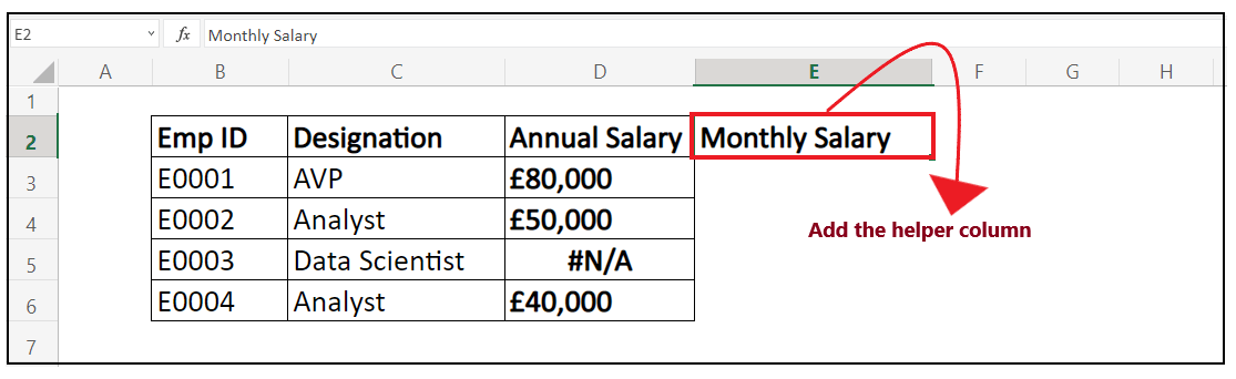
In this column we will type our IFNA formula and will trap #N/A errors for different data values. STEP 2: Type the IFNA formulaPut your cursor to the second row and start typing the function = IFNA( It will look similar to the below image: 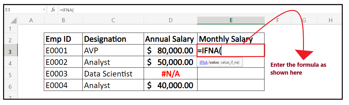
STEP 3: Insert the text parameter
It will look similar to the below image: 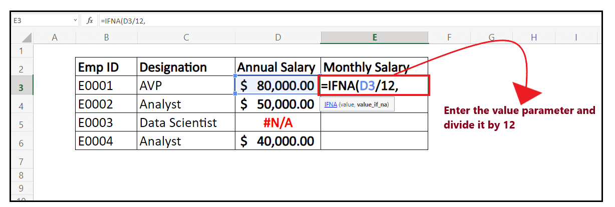
It will look similar to the below image: 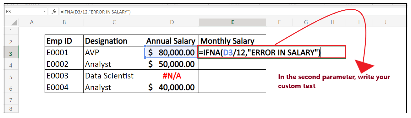
STEP 4: IFNA will return the resultSince IFNA has found no #N/A error, so it has returned the monthly salary by dividing the annual salary 12. It will look similar to the below image: 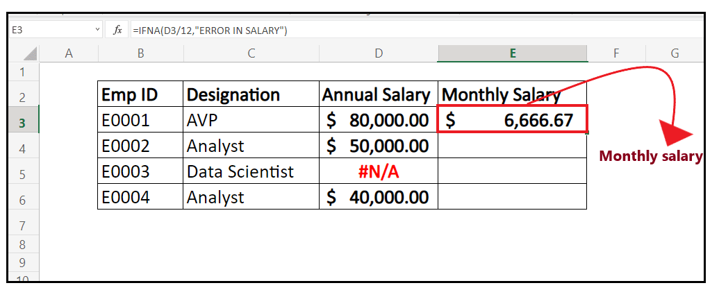
STEP 5: Drag the formula to other rows to repeat
It will look similar to the below image: 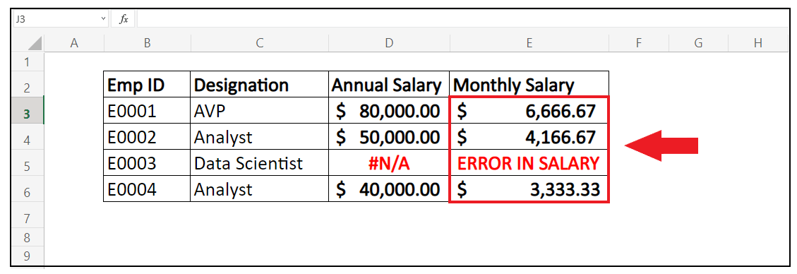
Next TopicExcel TRIM Function
|
 For Videos Join Our Youtube Channel: Join Now
Feedback
- Send your Feedback to [email protected]
Help Others, Please Share


