Microsoft Excel SUBTOTAL function with formula examples

What do you mean by the term SUBTOTAL Function in Microsoft Excel?

The Microsoft Excel basically defines out the SUBTOTAL as the Function that is responsible for the purpose of returning a subtotal in a list or a database. And in this context, the "subtotal" is not just used for totaling the numbers defined in a range of cells as it could be used for the other works too.

Unlike other Microsoft Excel functions that are primarily designed only to perform one if the specific thing, the SUBTOTAL function in Excel is amazingly versatile - as it can perform different arithmetic as well as logical operations which will be including the following things as well:

1. Counting of the respective cells.
2. Calculation of the average easily.
3. And the finding of the minimum or the maximum value in the given Excel sheet.

Moreover, the respective SUBTOTAL Function is readily available in all versions of Microsoft Excel, which are as follows:

• Microsoft Excel version 2016.
• Microsoft Excel version 2013.
• Microsoft Excel version 2010.
• Microsoft Excel version 2007, and lower version as well.

What are the basic points associated with the SUBTOTAL FUNCTION in Microsoft Excel?

The various key points that are associated with the SUBTOTAL Function in Microsoft Excel are as follows:

1. A subtotal function is basically considered as an inbuilt function in Microsoft Excel that is categorized under the Function: math or trigonometric function respectively.
2. The Subtotal will not just total out the numbers in a particular defined range of cells, as it will be helping out by performing out the various arithmetic operations on it.
3. And the SUBTOTAL Function in Microsoft Excel is very much versatile. And we can use it for the purpose of doing average, sum up, as well as counting a bunch of cells and the other calculations can also be performed efficiently.

Definition of SUBTOTAL FUNCTION

The SUBTOTAL function in Excel is primarily used for the purpose of returning a subtotal in a database or the list, that means finding out the Subtotal of a given range of particular cells.

SUBTOTAL Formula in Microsoft Excel

The formulas that can be used for the SUBTOTAL Function in Microsoft Excel are as follows:

Formula:

In which,

1. Function_num or operation code:The SUBTOTAL formula primarily indicates which respective Function should be used for the purpose of calculating the subtotals within a given list.

Furthermore, the function_num argument is applied based on the two criteria or methods as mentioned below.

1. Include hidden values: This value is basically used when the function_num argument is in between the range of 1-11, and the SUBTOTAL function will include the hidden values as well.
2. Ignore hidden values: When the function_num argument is in between the range of 101-111, and the SUBTOTAL Function will then exclude or ignore the hidden values. As it will be finding out values only invisible rows that ignore hidden values in the calculation.

1. ref1, [ref2]:It is termed as the one or more references to the particular cells containing the values on which the calculations need to be performed for the Subtotal as well.

What are the three top reasons to make use of the SUBTOTAL in Microsoft Excel?

Compared with the traditional Microsoft Excel functions, the SUBTOTAL Function eventually gives us the following advantages which are as follows:

1. Calculating out the values in filtered rows

The Microsoft Excel SUBTOTAL function ignores the values in filtered-out rows, which we can use to create a dynamic data summary in which the subtotal values are re-calculated automatically according to the filter respectively.

• For example: If in case we want to filter out the table in order to show the sales only for the East region, the Subtotal formula will be automatically adjusting it so that all other regions are removed from the total efficiently:

Important note.Because both function number sets (ranging from 1-11 and 101-111) will ignore filtered-out cells, we can use either the Subtotal 9 or Subtotal 109 formula in this case effectively.

2. Calculation of only visible cells in Excel sheet

It was made remember that, the respective Subtotal formulas with the given function_num 101 to 111 will ignore all hidden cells: filtered out and the hidden manually. So, when we are making use of the Excel's Hide feature in order to remove irrelevant data from a view, that in that scenario we can also make use of the Function 101-111 for the purpose of excluding the values in hidden rows from subtotals as well.

3) Ignoring all values in nested Subtotal formulas

Let us assume that, in a particular the range supplied to our Microsoft Excel Subtotal formula contains any other Subtotal formulas, and those nested subtotals will be ignored in that case, so the same numbers would only be calculated once.

In the below-attached screenshot, the Grand Average formula, that is: SUBTOTAL(1, C2:C10), will ignore the results of the Subtotal formulas in cells, that is, C3 and C10, as if in case we make Use of an Average formula with 2 separate rangesAVERAGE(C2:C5, C7:C9) respectively.

How to make use of the SUBTOTAL Function in Microsoft Excel?

Let us now look at how the SUBTOTAL Function works in Microsoft Excel.

# Example 1: SUBTOTAL Formula for values hidden making Use of the Excel Auto filter or Rows Hidden by a filter in Excel sheet

The respective table contains the Quarterly Sales Data in the below-mentioned example, in which the individual quarters are in column E and the sales data in column F respectively.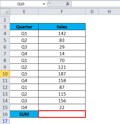

SUM FUNCTION is primarily applied in the respective cell "F16" =SUM (F4:F15).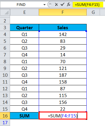

It will be returning or results in a value of1184, respectively.

Now the SUM function will return the same value that is none other than 1184, instead of 194 for the Q4 data if the rows are hidden by a filter (Below screenshot).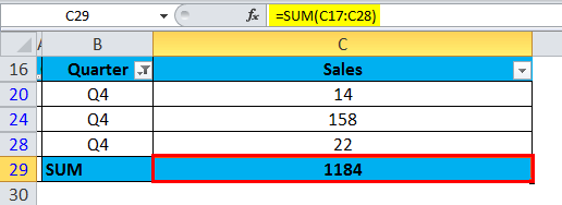

And if in case we want the Correct SUM value of Q4 data only, then in that case, we need to make use of the SUBTOTAL Function.

Now before applying the SUBTOTAL Function, that is present just under the data toolbar, we will be also applying a filter for the header row respectively.

So let us calculate specifically Q1 or Q2 or Q3, or Q4 sales data individually for filtered data:

We will be making use of the 109 as a function_num argument in the SUBTOTAL Function in order to summarize the data. i.e., =SUBTOTAL (109, C17:C28)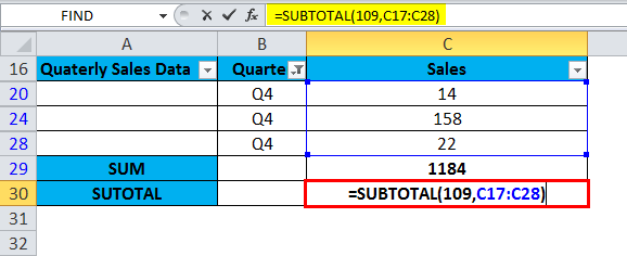

And the particular SUBTOTAL function will be then ignoring the rows hidden by a filter and calculating the correct result.

Here is the subtotal value that will get changes dynamically according to the filter. It will find only a sum of values in the visible rows, and the SUBTOTAL Function will neglect hidden rows as well.

Q4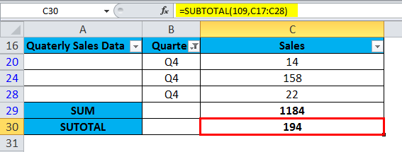

Q3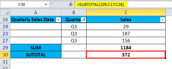

Q2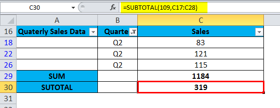

Q1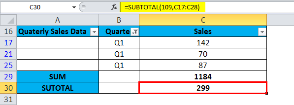

# Example 2:SUBTOTAL Function for the manually Hidden Rows in the Excel sheet

In the respective Microsoft Excel sheet, row no that is 15, 16, 19, as well as 20 have been hidden by making use of the row formatting option by just highlighting these rows, right-clicking with the help of the mouse, and after that, we will be selecting out the "Hide" option respectively.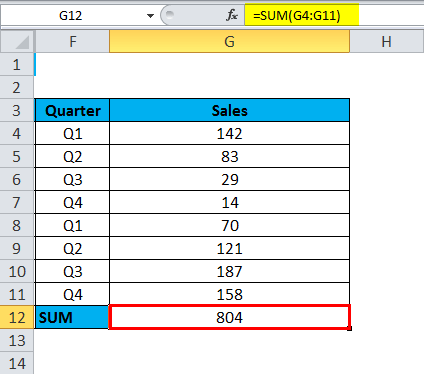

And a subtotal function is used in the respective cell that is C23 of the selected spreadsheet for the purpose of calculating the Sum of visible cells as well.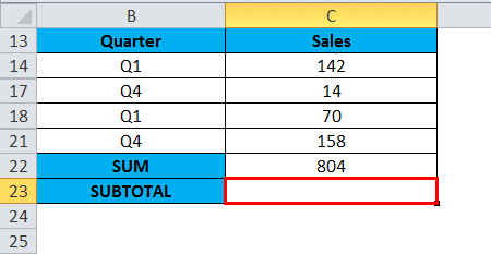

After that, we need to make use of 109 as a function_num argument in the SUBTOTAL Function in order to summarize the data.

i.e., =SUBTOTAL (109, C14:C21)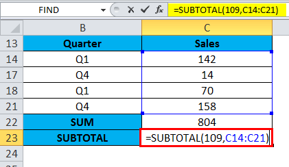

Here, the respective SUBTOTAL Function will then ignore rows manually hidden and calculate the correct result.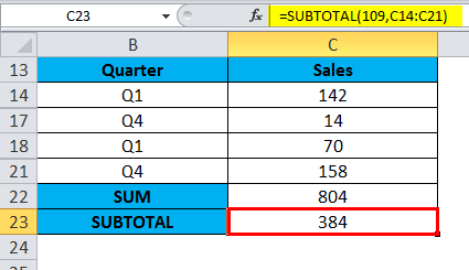

After that, it will find a sum of values in the visible rows only; the SUBTOTAL Function will also neglect the hidden rows.

# Example 3: SUBTOTAL Function for normal value in the Excel sheet

And in this, all of the selected cells in the given range of quarterly sales figures are visible, and none of them is filtered, or rows are hidden so that it will be including all the values.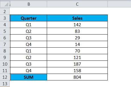

As in the below-mentioned example, we can see that multiple subtotal functions are easily applied.

So in the particular cell, C14, C15, and C16, SUBTOTAL Functions are applied efficiently.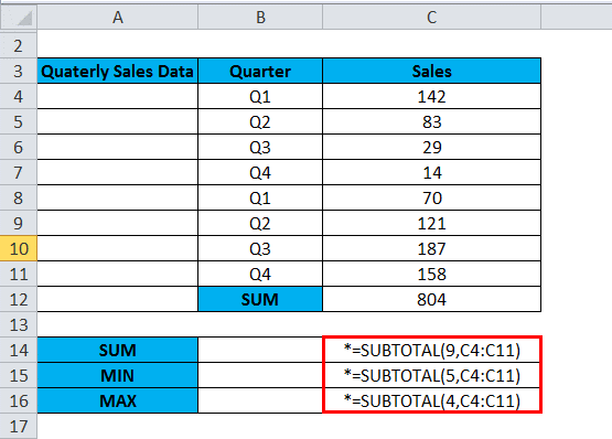

Now for the purpose of calculating the SUM value, the respective Function number that is either 9 or 109 is basically used in a subtotal function which will be then calculating the Sum of a specified range, that is:=SUBTOTAL (9, C4:C11).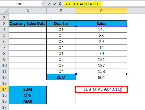

As soon as we apply the formula, it will give us the Sum of all values in the cell that is C4:C11, provided none are filtered, and the rows are hidden in that specified range.

And now, for the purpose of calculating out the MIN value, the respective Function number that is either 5 or 105 is used in a subtotal function where it will be finding out the smallest value in the specified range. In a particular cell, C15, a SUBTOTAL function is effectively applied, i.e. =SUBTOTAL (5, C4:C11):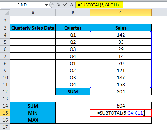

It will be finding out the smallest value in the given specified range that is from cell C4:C11:

And for the purpose of calculating out the MAX value, the respective Function number 4 or 104 can be used in a subtotal function in order to find the largest value in the specified range. And in a cell, C16, a SUBTOTAL function is applied, that means=SUBTOTAL (4, C4:C11):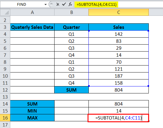

It will then find out the largest value in the specified range from C4:C11, respectively.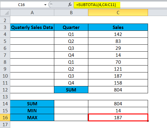

Microsoft Excel Subtotal not working: common errors

If in case our respective subtotal formula returns an error, it is just likely to be because of one of the following reasons as well:

1. #VALUE!: And the particular function_num argument is other than an integer that is ranging in between of 1 - 11; or any of the ref arguments containing 3D Reference.
2. #DIV/0! It primarily occurs if a specified summary function has performed a division by zero.
3. #NAME?: The name of the respective Subtotal Function is misspelled - then the easier error needs to be fixed respectively.

Important note: It should be noted that if we do not feel comfortable with the SUBTOTAL Function yet, we can use the built-in SUBTOTAL features and have the formulas inserted for us automatically.

What are the important things which need to be remembered by an individual in Microsoft Excel?

The important things that need to be remembered by an individual while working with the SUBTOTAL Function in Microsoft Excel are as follows:

1. An individual can effectively apply a respective SUBTOTAL function for the purpose of finding out a sum of filtered values.
2. And the particular SUBTOTAL function is primarily used for the purpose of ignoring out the values in the hidden rows respectively.
3. Moreover, the unction _ num argument value must not get exceed by 11 or less than 1 in any of the case. Similarly, it should not be greater than 111 or less than 101; if it is greater than the value mentioned earlier, then in that scenario it will be giving an error: #VALUE! Error.
4. And a SUBTOTAL function is primarily applicable only for the numeric value only.
5. And if in case any subtotals are usually present in the SUBTOTAL range, then, in that case, they all will be neglected, which means that if any already existing SUBTOTAL formulas are there in the input range of other SUBTOTAL formulas, then that particular values are neglected by the subtotal Function during the calculation so that the occurrence of the double counting is avoided and thus preventing out the error of double counting as well.
6. Besides all these, a SUBTOTAL function can efficiently use for the purpose of summarizing out the data dynamically.
7. And the Blank cells as well as the cells which are containing the non-numeric values are ignored by the subtotal Function during the calculation effectively.