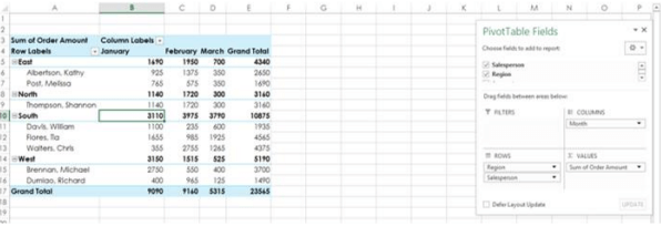
Pivot table in Excel 2011

Pivot table is a tool provided by MS Excel that enables the user to slice and dice the data stored in the spreadsheet.

It allows the user to study the data from various data points and then modify it dynamically, giving a new perspective.

Some of the features provided by the pivot tables are churning, sorting, and filtering the data. You can generate multiple reports using the pivot table in less time. You can also select a representation to gain insights from the data. It increases the efficiency of working with the data.

Creating a Pivot Table in Excel 2011

If you want to create a Pivot table in MS Excel, then the first step is to select the range of data with which to create the table.

The user can also begin with an empty Pivot table and then fill in the data in that pivot table.

The user can also use some of the Recommended Pivot tables in MS Excel. These will give you an idea of the table's layout, and you can choose the best way to summarize and represent the data.

In MS Excel, you can build a pivot table from multiple tables or different data sources. You can also use external data sources to create the pivot table of the data.

A pivot table that uses its database is called PowerPivot, and the database is known as the data model.

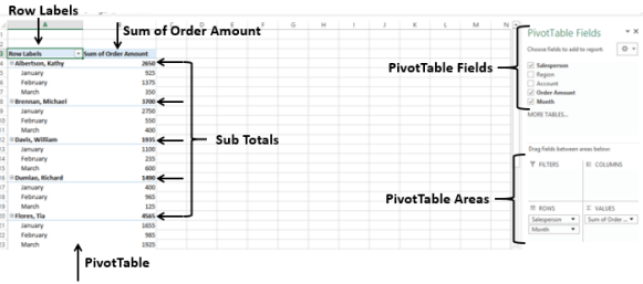
Pivot Table Layout-Fields and Areas

The Pivot table layout depends on the fields you have chosen to import the data for reports. The layout can also be affected by the arrangement of the data in the Areas. You can choose the data or the arrangement by dragging the data fields. As you drag the fields in the pivot tables, the layout of the Pivot table will automatically change.

Exploring the Data with Pivot Table

The Pivot table is a powerful tool. It enables the user to quickly extract the important data in the spreadsheet. The whole objective behind using this tool in MS Excel is to effectively explore the data stored in the spreadsheet.

It also provides the user to effectively manage the data. The user can use options such as Sorting, filtering, collapsing, expanding, and grouping or ungrouping the data.

Summarizing the Values in the Pivot Table

In MS Excel, the user has various types of calculations. The user can use these calculations according to the need and suitability of the data entered in the Pivot table. The user can also change different calculations. Once you have prepared the data in the Pivot table, after collating the data by using different exploration techniques, the user can move to the next step, which is to summarize the data. The results are also displayed simultaneously.

Updating the Pivot Table

Once you have studied the data in the pivot table, the user can summarize the data. The user does not require to perform the above step again. Once the data in the pivot table is modified, you can just refresh the table, which will automatically reflect the changes in the Pivot tables.

Once you have prepared the summary for the data, the last step is to represent the data in a Pivot table. The user can create interactive reports using the data stored in the Pivot table. The reports created using the data in the pivot tables are also dynamic. The user can easily modify or change the perspective of the data present in the report. The user can determine the report based on the detail and information required. It also allows one to choose the focus on certain items in the audience's expressed interest.

Creating a Pivot Table from a Data Range

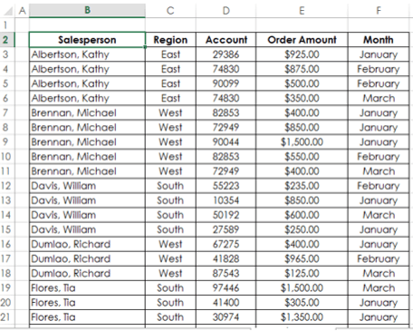
The first step is to ensure that the first row has headers. This is necessary as these headers will serve as the headings in the pivot tables.
Give a name to the data range you want as your pivot table's data source.
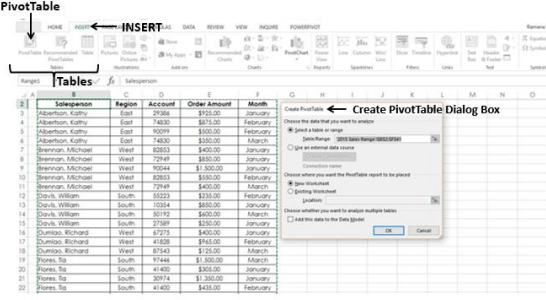
Click on the data range.
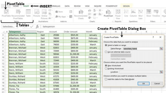
Click on the Insert tab in MS Excel. Select the Pivot table.
This will open a dialog box allowing you to create a Pivot table.
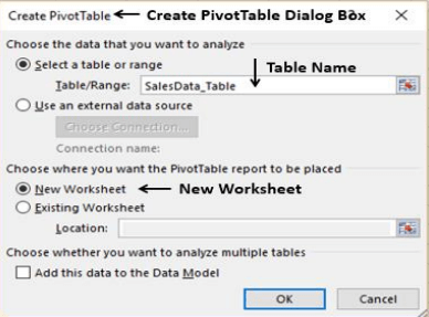
In the dialog box, the user can choose the data that the user wants to be added as the pivot table. The user can either select an entire table or can only select a range in the table.
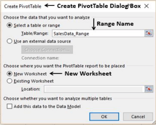
We want to select the data range as the source for creating the pivot table.
From the dialog box, click on Select a table or range, then in the table/range box, enter the name of the data range.
Select New Worksheet under the section where you want to add the Pivot table report to be placed in your spreadsheet.
Then click on OK.
The user can also study multiple tables simultaneously. To do so, select Analyze multiple tables after adding the data range in the Data model.
The above step will add a new worksheet to the workbook. This worksheet will contain an empty pivot table in the worksheet.
Assign a name to the worksheet.
The fields of the pivot table will appear on the right side of the worksheet. It contains all the names of the columns in the data range.
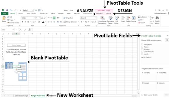
Go back to the Insert Ribbon from the Pivot table tools - Analyze and design appear.

Adding the Fields in the pivot table

Click on a field in the Pivot tables from the list of fields and drag the selected field into the row area.
Select the other field that you want to include in the summary, and drag that column in the Rows area.
Now click the values inside the field and drag that into the summation value area.
Thus, your first pivot table will be ready.
Once the pivot table is constructed, go to the end of the worksheet. You will see a row marked as the Grand total containing the total sales.

Creating a Pivot table from a table

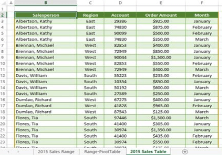
In MS Excel, a table already has a name, and the columns have headers.
To create a pivot table in the spreadsheet, select the table that you want to use as the data source for the table.
After selecting the table, open the Insert tab from the Excel ribbon.
Select the pivot table from the tables group in the insert tab.
This will open a dialog box that enables the user to create the Pivot table.
Now, go to select a table or range. From the menu, go to the Table/Range box and enter the table's name in the dialog box.
Now, open a new worksheet. This will be the worksheet in which the pivot table report will be displayed.
After finalizing the worksheet in which you want to place the worksheet, click on OK.
This will add a new worksheet to your workbook, and this new worksheet will contain an empty Pivot table.
Add a name to the spreadsheet.
The pivot table will be ready.

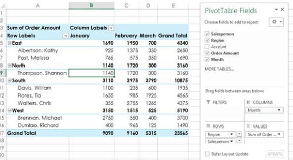
Fields in Pivot tables

The fields in the pivot table are similar to a task pane. The fields are related to the pivot table in the spreadsheet.
The pivot tables combine task panes known as Fields and Areas. The fields of the pivot table are displayed above the areas. The task pane is default displayed on the window's right side.
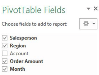
The fields of the pivot table show the columns that store the data in the table. The column of the pivot table is the same as the column in the range or excel table.
The columns inside the table will appear with check boxes against them.
The fields chosen by the user will be displayed in the report.
The areas determine the orientation of the report. It is the layout that also includes the calculations performed in the report.
You will have an additional option below the task pane in MS Excel to Defer the Layout Update of the report by using the Update button.
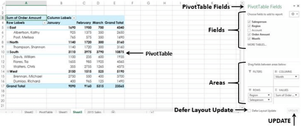
By default, if you won't select the option mentioned above, the modifications made in the fields you selected or in the layout of the report will be performed in the pivot table instantly.
But once you select the above option, modifications in the selected field will be implemented in the fields only when the user Updates the report.

Pivot table Field Task Pane

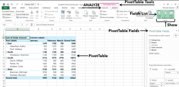
The pivot table field task pane is located in the worksheet in which you have placed the pivot table.
If the pivot table field task pane is not visible in the worksheet. Then follow the following steps to view the Pivot table Fields task pane.
Select the pivot table in your worksheet.
If the pivot table fields task pane is not displayed in the worksheet, then go to the insert ribbon.
Select the analyze tab from the pivot table group. It is located under the Pivot table tools.
Check if the columns of the pivot tables are selected in the Show group.
If the column of the pivot table is not selected then select the field by clicking on the field from the Fields list.
The pivot table fields task pane appears on the right side of the MS Excel application. The pivot table fields task pane is under the title Pivot table fields.

Moving Pivot table Fields Task Pane

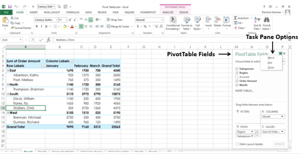
To the right of the title Pivot table Fields in the Pivot table task pane, you will see a button with an arrow pointing downwards. Click on the button.
It will open a list of options you can perform on the pivot table. These are move, size, and close. The options will be in the drop-down menu.
You can change the location of the task pane of the pivot table by moving it to the location you want it to. To move the task pane, you need to follow the given steps:
Select move from the list of options in the drop-down menu.
A button will appear on the pivot table task pane. Select the icon. This will enable you to drag the task pane to where it should be.
The user can place the task pane's location anywhere in the worksheet.

Changing the Size of the Pivot table Fields Task Pane

You can increase or decrease the length and width of the pivot table task pane by following the given steps.
Open the task pane options. To select from the options, click on the button right to the title of the pivot table fields. Select the option to size the pivot table task pane from the drop-down menu.
a symbol will appear that enables the user to increase or decrease the length and width of the task pane.
Sometimes, the value is not completely visible in the task pane. To prevent this, you can resize the task pane.

Pivot table Fields

The pivot table field consists of the tables that are constructed in the workbook. It also includes the tables that are related to the corresponding field.
If you want to create the pivot table, you will have to determine and choose the fields from the Pivot table fields list.
This will create a pivot table structure with all the fields selected in the previous step.
The user can anytime select or deselect the fields anytime. This will change the Pivot table. The fields with corresponding boxes checked will appear in the table. Once the pivot table is created, the data is entered.
The user can highlight the summarized data that the user wants to present in the report.
If a single table exists in the spreadsheet, then the table name will not appear in the pivot table field list.
Only those fields with checked boxes against them will be displayed. On the top of the field list, you can find the action to select the fields for adding to the report.
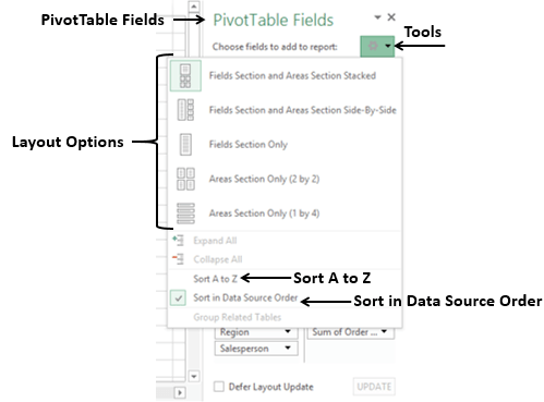
on the right side of the field, the user can see the button that shows Tools.
Right-click on the Tools button. This will open a list of the user's tools in the table. From the drop-down list, the user will see the five different layouts option available for fields and areas.
Two sorting options are available to arrange the field list in the pivot table.
Sort from A to Z
Sort the Field in Data Source Order
The sorting order is default set to Data Source order. This sorts the data in the same order the fields are arranged in the column in the data table.
The user can sort the fields of the pivot table in alphabetical order. The user must click -Sort A to Z from the drop-down menu in the tool list.