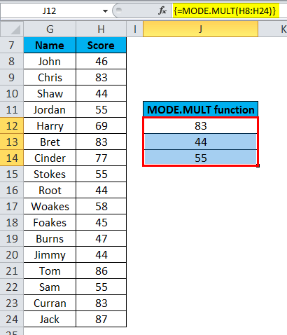
Mode Function in the Microsoft Excel

We often use MODE in mathematical stats calculation. The same concept is used in Microsoft Excel as well. This tutorial will cover the step-by-step implementation of the Excel Mode Function.

What is MODE Function?

"The Mode function in Microsoft Excel is the other most important function that will allow only numbers to be used effectively as it was categorized under the Microsoft Excel statistical functions. And the respective Mode function in Microsoft Excel is purposely used for calculating the most frequently used or the occurring values from the particular list of the supplied data."

The function will return the lowest from the given set of values (lowest of the values). Furthermore, the MODE function can be efficiently used in the respective financial analysis to calculate the mode for the given data set accurately. For example, we have a dataset of millions of people. We can assign the numbers to the individual making purchases like the Television (T.V) =1, Mobile phone =2, similarly Tab =3. Then in these cases, the data can be serves as an important as well as a valuable marketing tool. With the help of the mode function, we can quickly figure out how frequently consumers are interested in buying the above gadgets.

Now take the other example; in this particular example, let us assume that if there are 3 cells in the specific range out of which the 3, 2 cells contain the same number, then the Mode function will return that number which is repeated two times. And if all the 3 cells have different numbers, then we will encounter an error message that is none other than #N/A, as we all know that the Mode Function could not return anything.

Using the MODE Formula in the Microsoft Excel:

We have attached the screenshot of the Mode Formula that can be effectively used in Microsoft Excel:

Explanation of the Mode Function in the Microsoft Excel:

Moving further, we will explain the Mode Formula an individual uses in Microsoft Excel according to their needs.

The MODE Formula, which is actively used in Microsoft Excel, has the below-mentioned arguments, which are discussed in brief:

1. number1 (compulsory OR the required idea): It was known that the Arrays of the respective cell reference or the numeric values (which are the set of one or more numeric values) for which we need to calculate the mode efficiently.
2. number2 (Optional OR not required): In these, the Arrays of the particular cell reference or numeric values (which are the set of one or more numeric values) for which we need to calculate the mode respectively.

Besides these, it was noted that the 255 numbers could be efficiently supplied as separate arguments.

Points to Remember

For the particular Mode Function, we should know the following points that are as follows:

1. The Arguments can either be the particular numbers or the names of the arrays, or they could be the references that contain the numbers.
2. And if an array or the particular reference arguments contain the text, the logical values, and the empty cells, then, in that case, the values are ignored by the function mentioned above (Mode Function). Moreover, any cells in the Microsoft Excel sheet with zero (0) are included.
3. And the arguments containing the error values or the text that cannot be translated into numbers may cause the errors.
4. The MODE.SNGL function in Microsoft Excel returns the single-mode, which considers the repetitive numeric value.
5. The MODE. The MULT function is responsible for returning the vertical array of the most frequently occurring or repetitive values in an array or the range of data.
6. And to return out the horizontal array, then, in that case, the transpose function is added along with MODE.MULT function respectively which means that the TRANSPOSE(MODE.MULT(number1,number2,?))

How do you make Use of the MODE Function in Microsoft Excel?

It was assumed that the particular MODE Function in Microsoft Excel is considered a straightforward and easy-to-use function. Now let us understand the working of the MODE Function in Microsoft Excel with the help of the various MODE Formula and examples.

# Example 1:

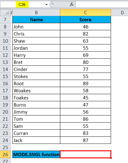
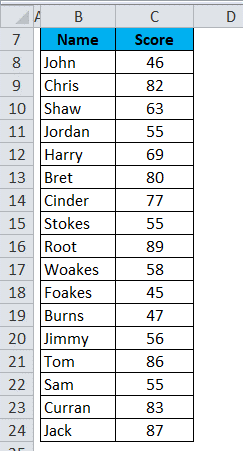
As in the below-mentioned example, the respective Table contains the Name of the student in column B from B8 to B24 and, similarly, the score of each student in column C from C8 to C24. And here, in this, we need to find out the most frequently occurring or the repetitive score or the particular value in the range of the data with the help of the MODE.SNGL FUNCTION effectively. As can be seen in the below-attached screenshot,

Follow the below steps to apply the MODE function for the above data set:

1. Select a cell in which you want to apply the MODE.SNGL function to fetch the results, as clearly depicted in the screenshots below.
   
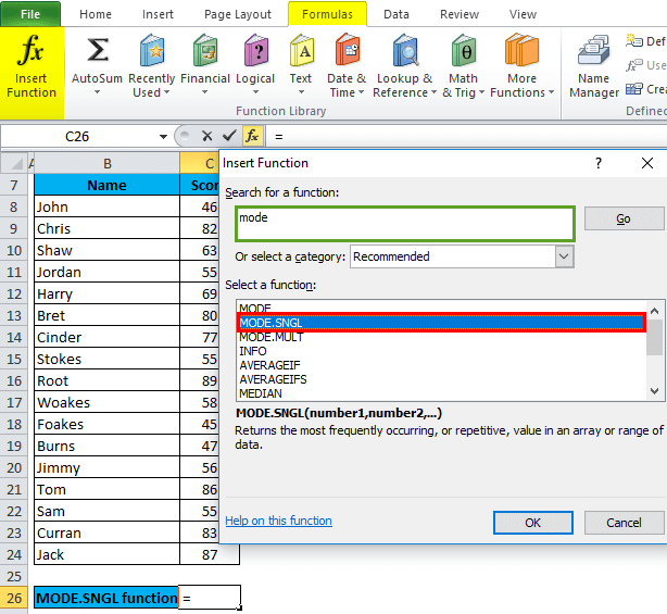
2. Click on the insert function button (fx), which is present under the formula toolbar; as soon as we click on the insert function button, a dialog box will get appears on the screen; in which we will be typing out the keyword that is the "MODE" in the search for a function box.
3. The MODE function is used for Microsoft excel 2007 as well as in the earlier version too. So, we must need to select the MODE.SNGL function. And make Double-click on MODE.SNGL function, respectively, as it is depicted in the below-mentioned image.
   
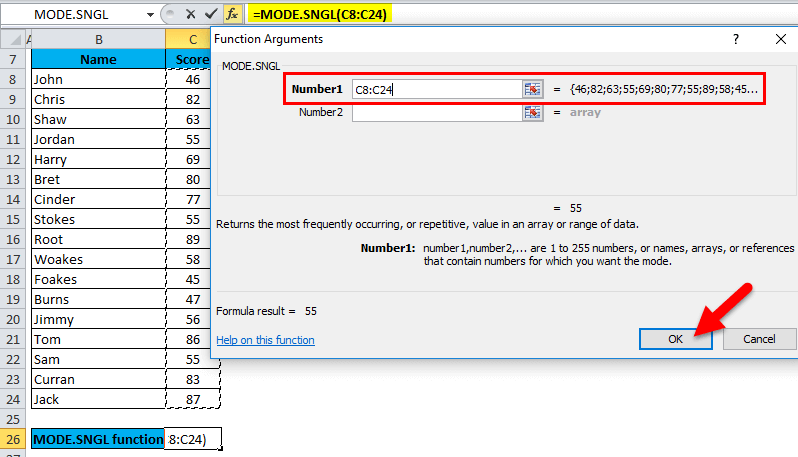
4. The dialog box will appear, fill the arguments of the MODE function. =MODE(number1, [number2], ? respectively,
5. And to enter the Number 1 argument, we will click inside cell C8 and see that the particular cell will be selected effectively; then, we will determine the cells until column C24. So, the column range will be chosen from columns C8: C24. And then, we will click on the "OK" button, as seen in the figure below.
   
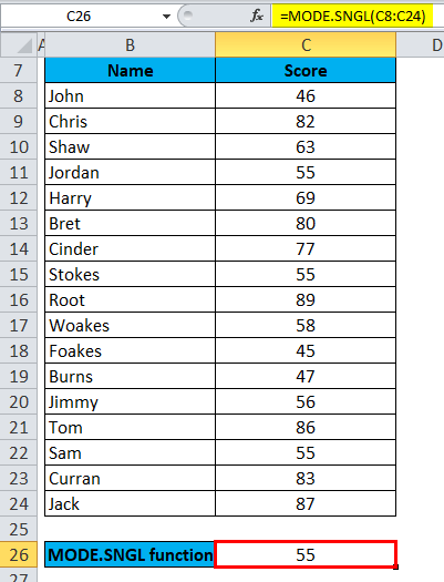
6. Soon after entering out the number1 argument, = MODE(C8:C24), which will return the most frequently occurring or the repetitive score or value 55 as the outcome or the value in the respective cell C26, as it is depicted in the below-mentioned image.
   

#MODE Example 2:

MODE.MULT functions in Microsoft Excel will return more than one result or the outcomes, and if in case multiple ways are entered as an array formula, then let's check out this with the help of the below-mentioned example.

As the below-mentioned Table contains the Name of the student in the column that is the "Name column" from column G8 to column G24 and then the score of each particular student from column H8 to column H24, and here in these, we need to find out the most frequently occurring as well the repetitive score in the range of data by the help of MODE. MULT FUNCTION, as is seen in the below-attached screenshot.

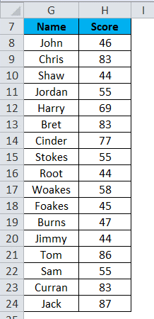
Now, here in these, we need the repetitive score for more than one occurrence, which means the MULTIMODE, so for these, we need to use the array formula to operate on the various available multiple values instead of the single value.

1. Select the cells from cells J12 TO J14, where MODE.MULT is applied efficiently, as seen in the screenshot below.
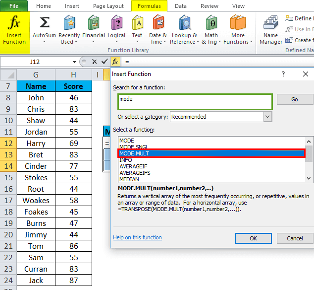
2. Click on the insert function button (fx), which is present under the formula toolbar; as soon as we click on the insert function button, a dialog box will get appear on the screen; in which we will be typing out the keyword that is the "MODE.MULT" in the search for a function box.
3. Select out the respective MODE.MULT function to make a selection of the function box, and soon after that, click on the MODE.MULT function. As can be seen in the below-attached screenshot,
   
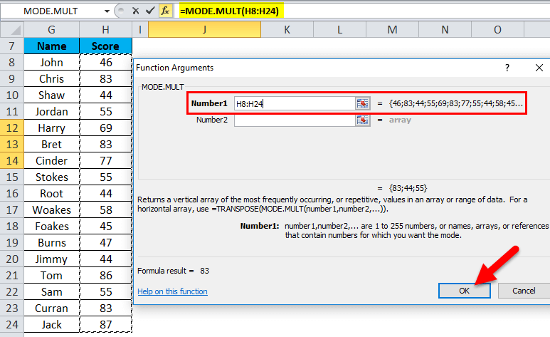
4. After that, a dialog box will get appears where arguments for MODE will be.MULT function must be entered out or fill in the particular box, which means the =MODE.MULT(number1, [number2], ? respectively,
   =MODE.MULT (H8:H24)Here, the score data is primarily present in the range from H8 to H24, for which we must apply the MODE.MULT function efficiently.
5. Enter the Number 1 argument, we will click inside cell H8 and see that the particular cell will be selected effectively. Then we will select the cells till cell H24. So, the column range will get chosen from columns H8: H24.
6. Click on the "OK" button respectively, as can be easily seen in the below-attached figure.
   
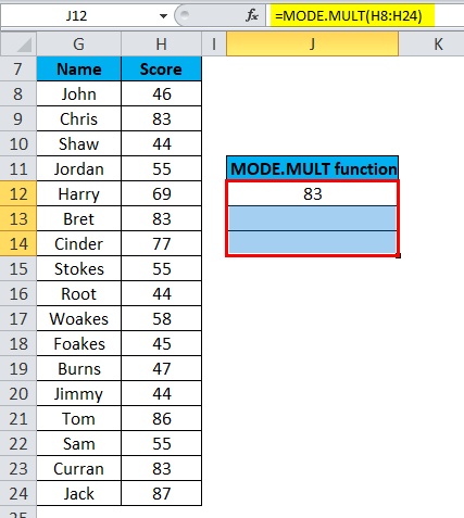
7. And after performing the above, we will get the result or the outcomes as seen in the screenshot below.
   
8. And now, after entering the number1 argument.
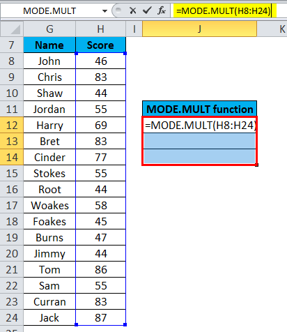
9. Highlight the particular range of cells for the given function result to apply an array formula from H8 TO H24. And to stress, we will be clicking on the formula toolbar. So automatically, the range H8 TO H24 and J12 to J14 cells gets selected for an array, respectively, as seen in the screenshot below.
   
10. Now click on Ctrl + Shift + Enter so that output values of the respective MODE.MULT returns in cell J12 to J14.
11. The array formula that is applied will appear as {=MODE.MULT (H8:H24)} in which the MODE.MULT in the formula bar is encased in curly braces { }.
12. MODE.MULT returns more than one result. i.e., 83, 44 & 55, as can be easily seen in the screenshot below.
    

Things to Remember

Various essential things need to be remembered by an individual while working with the Mode Function in Microsoft Excel as follows:

1. In the Microsoft Excel 2010 versions, the MODE function is replaced by the other function, such as the MODE.SNGL; the current versions of Microsoft Excel still provide the MODE function to allow compatibility with the earlier versions. And it was known that the MODE function is primarily stored within the list of the various compatibility functions. However, the MODE functions may or may not be available for future versions of Microsoft Excel, so an individual should use the MODE.SNGL function whenever it is possible.
2. #NUM! Error: It must be remembered that the #NUM! Error get appears or occurs if there are no respective duplicates available, and hence, there is no mode within the available supplied values respectively.
3. #VALUE! Error: The #VALUE! The error usually gets if the particular values supplied directly to the MODE are non-numeric and are not part of an array. And the non-numeric functions, which are part of the specific array of values, are effectively ignored by the MODE Function.