Cell References in Excel

MS Excel or Microsoft Excel is powerful spreadsheet software developed by Microsoft. Each worksheet in Excel consists of several cells formed by rows and columns. Each cell has a specific reference (or cell reference) which helps the users easily access/address the desired cell (s) within the functions. Cell references play an important role in Excel, especially when using functions and formulas with large data sets.

In this tutorial, we discuss a brief introduction to Excel Cell References. The article also discusses the different types of cell references available in Excel and the step-by-step procedures for using the respective cell references.

What is a cell reference?

A cell reference refers to the name or address of a specific cell or range of cells within the spreadsheet. A cell reference is commonly used as a variable in Excel formulas. While representing the cell reference in Excel, we need to specify the column name followed by the row number of the respective cell.

The following image displays the cell reference of the selected cell in an Excel sheet: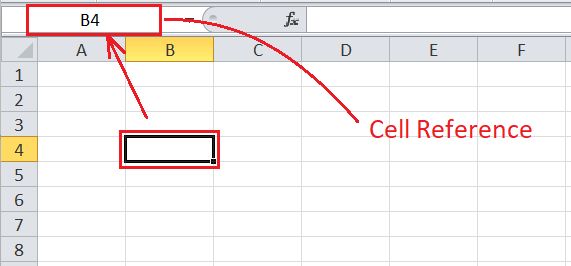

Cell reference mainly helps the Excel program locate the cell within the sheet and read or use its data in the specified formula to generate the result. We can use cell references or a range of multiple cells in other cells when creating a formula, even if the corresponding cell is on the same sheet, different sheet, or different workbook.

In Excel, cell referencing uses values or properties of another cell or range in a different cell/range. When referencing cells from other worksheets, this is usually called external referencing. When cells are referenced from other spreadsheet programs, it is referred to as remote referencing.

Let us now understand simple examples of using cell references in Excel:

A Simple Reference

The basic use of a cell reference can be displayed by simply mentioning the referred cell with the equal sign. For example, if we enter "=A1" without quotes in another cell within the sheet, the value of A1 will be displayed in the corresponding cell. This means that the value of the selected cell, where the cell reference is entered, is exactly equal to that of cell A1.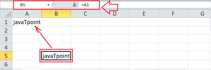

Reference to a Cell Range

We can also use the reference of multiple cells at once by referring to their cell range. For example, if we use the notation "=A2:C6" without the quotes, we refer to the entire cell range from A2 to C6. However, a range alone is not valuable data in Excel. When we use this cell reference in an Excel cell, Excel gives the #VALUE! error, which means that the formula is missing. Therefore, a reference to a cell range (A2:C6) has meaning only when used within a function or formula (as discussed next).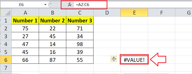

Cell Reference in a Function

Excel can perform a tremendous job when we use a cell range in a function. For example, if we supply the range A2:C6 in SUM function, Excel adds up all values of the cell range from A2 to C6 gives the calculated value as a result.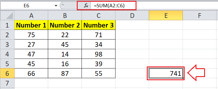

Similarly, if we supply the same range (A2:C6) to an AVERAGE function, Excel returns the average of the corresponding cell range, as shown below: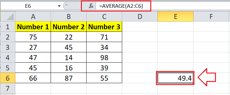

In this way, we can leverage cell references in Excel and perform various operations or calculations on the recorded data within the cells. There are different ways to use cell references in Excel, depending on the use cases.

How many types of cell references are there in Excel?

Understanding different types of cell references mainly help us to work with Excel formulas easily, thereby preventing unexpected formula errors. This is most helpful when copy-pasting Excel formulas. There are three primary types of cell references in Excel based on different use cases, such as:

• Relative Cell Reference
• Absolute Cell Reference
• Mixed Cell Reference

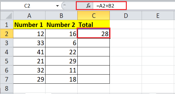
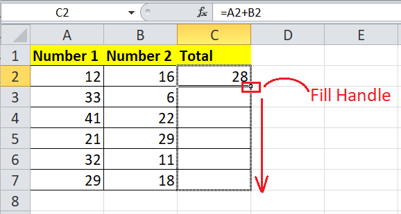
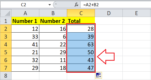
Let us discuss each type of cell reference in detail:

Relative Cell Reference

A relative cell reference is the default approach in Excel. Whenever we enter any cell reference or a range within the formula in Excel, the reference used is relative. The corresponding cell references are used normally with the relative references, which typically represent the combination of column name and row number. The cell reference does not contain any dollar ($) sign in relative reference.

When we copy formulas from one relative cell to others, the cell references are automatically adjusted by Excel based on respective rows and columns. The relative cell references are commonly used to perform the same operation on multiple relative cells by changing the corresponding cell's column and row addresses in the formula.

How to use relative cell references in Excel?

Suppose that we have the following Excel sheet with two numbers in columns A and B, and we want to add both the values in column C.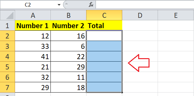

We need to perform the following steps to use a relative reference and sum up values from the same rows of columns A and B.

• First, we must select the destination cell to enter the formula to add values. In our case, we select cell C2 and enter the formula "=A2 + B2" without quotes. After that, we press the Enter key to get the calculated value in cell C2.
  
• Next, we must copy-paste cell C2 to other relative cells from C3 to C8. Alternately, we can click and hold the fill handle from the bottom-right corner of cell C2. We must drag the fill handle to the last cell we want to copy the respective formula. In our case, we drag the fill handle to cell C8.
  
• After copying the formula to all corresponding cells from C3 to C8, the addition operation is performed using values from cells A3, B3, and A4, B4, etc.
  
• We can select any destination cell and check the applied formula from the formula bar. For instance, if we select cell C5, we can see that the addition is performed between cells A5 and B5.
  
  In the above image, it is clear that the relative address of cell A2 changes to A5 and B2 to B5. Similarly, the relative addresses of other cells also change accordingly based on the relative position of the respective row and column.

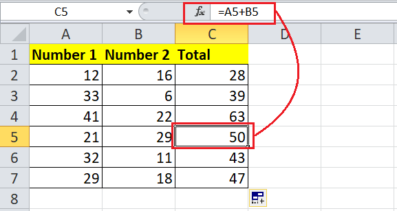
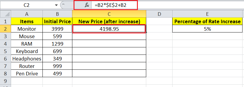
It is important to note that we can use cell references as normal when dealing with relative references.

Absolute Cell Reference

In Excel, we don't always want Excel to automatically change the references, especially when copied into other cell or a range that are not relative. In such cases, the formula gives wrong results or the formula error. This is where the absolute cell references are useful. Unlike relative cell references, absolute cell references do not change when copied to other cells.

An absolute reference is the cell reference in which the corresponding reference is locked, meaning that the row and column remain constant. This type of cell reference contains a dollar ($) sign before the column name and row number, making the corresponding reference fixed. We can press the F4 function key to fix the reference or lock it for the selected cell. $A$1, $B$1, and $C$1 are examples of absolute cell references.

How to use absolute cell references in Excel?

Suppose that we have the following Excel sheet with some items (Column A) with their initial prices (Column B). However, the prices have increased by 5% (cell E2), and we need to calculate the new price for each item using the absolute cell reference.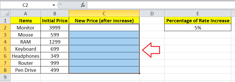

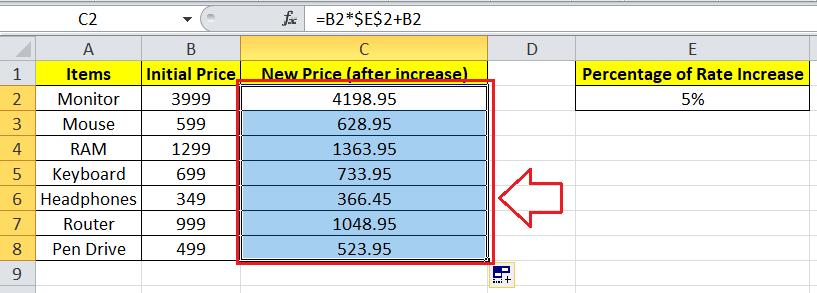
We need to perform the following steps to use an absolute reference to calculate increased prices (Column C) for each item:

• First, we must select the destination cell and enter the formula to calculate the new/increased price. In our case, we select cell C2 and enter the formula "=B2*$E$2+B2" without quotes. After that, we press the Enter key to get the increased price in cell C2.
  
  According to the formula above, we multiply the item's initial price with the increased percentage rate and add the resultant value to the old price for the respective item. In this way, we can calculate the increased price of the item.
• Since the increased rate percentage is fixed (5%) for each item, we add the dollar ($) signs with E2 cell to make it absolute, i.e., $E$2. Thus, $E$2 will be unchanged after copying the formula into other cells.
• Next, we must copy-paste cell C2 to other relative cells from C3 to C8. Alternately, we can click and hold the fill handle from the bottom-right corner of cell C2. We must drag the fill handle to the last cell we want to copy the respective formula. In our case, we drag the fill handle to cell C8.
  
• When copied the formula into other relative cells, the values from column B change automatically. However, the absolute reference ($E$2) does not change. For instance, if we select cell C5, we can see that cell B2 has changed to B5, but $E$2 is constant.
  

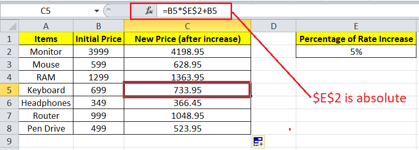
It is important to note that we must use the dollar ($) sign in both row and column letters to create an absolute cell reference.

Mixed Cell Reference

As the name suggests, the mixed cell reference combines the relative and absolute reference. The dollar sign is used either before the column letter or the row number in a reference. With the mixed reference, we can use the following two cases in reference:

• The column remains fixed, while the row changes as the relative reference when copying the respective formula.
• The row remains fixed, while the column changes as the relative reference when copying the respective formula.

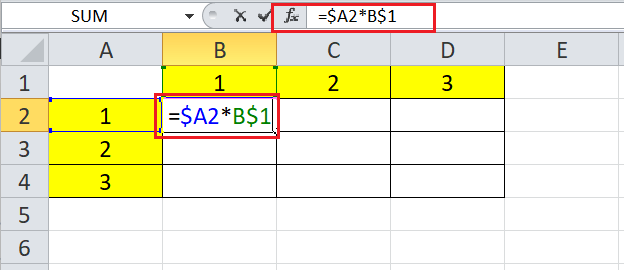
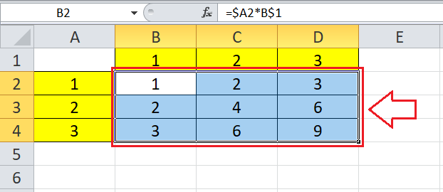
$A1 and B$1 the examples of the mixed cell reference where relative and absolute references are combined.

How to use mixed cell references in Excel?

Suppose that we have the following Excel sheet with some values in cells A2, A3, A4 of column A and cells B1, C1, D1 of the first row. We need to multiply each column cell with each respective cell of the row using the mixed cell reference.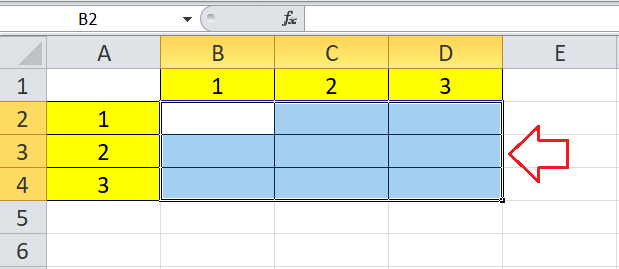

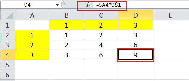
We need to perform the following steps to multiply each column with each row by using the Mixed Cell Reference:

• First, we need to select cell B2 and apply the formula "=$A2*B$1" without quotes. The first parameter ($A2) represents the absolute column and relative row. This means that column A is locked, while the row number can change. The second parameter (A$2) represents the absolute row and relative column. The first row is fixed, while the column can change.
  
• Next, we need to copy the same formula to all the cells of the range B2:D4. Instead of entering the formula in each cell, we can select an entire range and click 'Ctrl + D' and 'Ctrl + R'. This will apply the formula in all the selected cells and generate the results accordingly.
  
  If we select cell D4, we can see that column A is constant in the first parameter ($A4), and row 1 is constant in the second parameter (D$1).
  

It is important to note that either row or column is made constant to create absolute cell reference.

Important Points to Remember

• The cell reference is one of the key elements for Excel functions or formulas.
• The cell references can be used with functions, formulas, charts, and many other essential commands present in Excel.
• When relative cell references are used in Excel formulas, the references are adjusted automatically as per the corresponding row and column.
• It is recommended to use absolute cell references when copying formulas in cells that are non-relative. The absolute cell references do not change by Excel.
• Mixed reference locks only one of the references, either row or column, as per requirements. It does not lock both.