How to cut characters in Excel

How to remove characters in Excel?

Data entered in the worksheet sometimes needs to be edited based on the requirement. If the editing work is limited to small data, the work is simple and done faster. But what if the large data needs to be edited? Editing large data manually takes a lot of time and is tough. Editing work includes extracting or parsing certain characters without changing the given data and replacing certain characters with the specified data. Excel provides various methods and formulas to change the data present in the cell. In this tutorial, the various methods are explained.

Example 1: How to cut the specified text using Find and Replace?

In this example1, the specified text is removed using the Find and Replace Method. As the name suggests, it finds and replaces the selected text with specified text. It does the work quickly and efficiently, which saves time. The steps to be followed are,

Step 1: Enter the data in the worksheet, namely A1:A10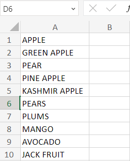

Step 2: Select the range of cells to replace the specified text.

Step 3: Here, the cell range A1:A10 is selected. Click Ctrl+H. The Find and Replace dialog box will open.

Step 4: The word APPLE needs to be removed from the data. Hence in the FIND dialog box, enter the data as APPLE. The Replace dialog box should be left empty. Click Replace ALL.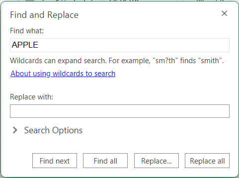

Step 5: The word APPLE is removed from the data using the Find and Replace function.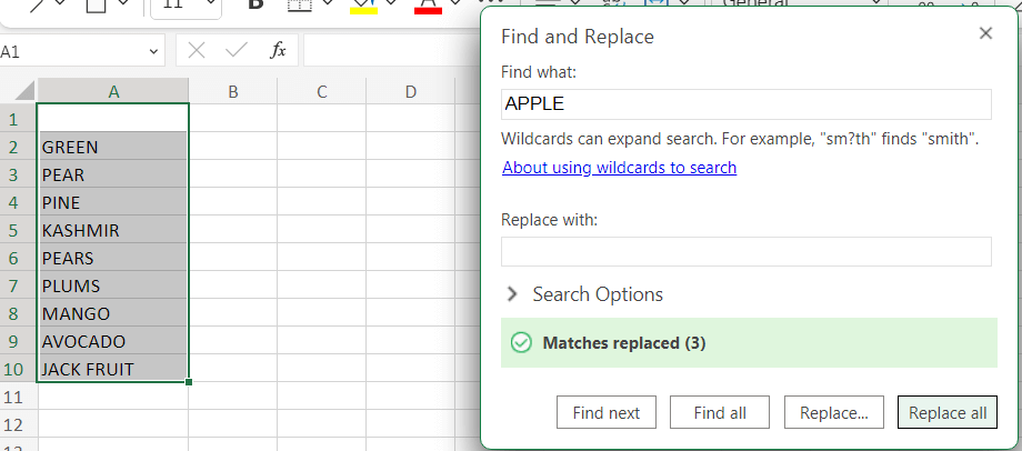

In the worksheet, three matches are replaced in the given data.

Example 2: How to cut the specified symbol in the given data?

In Example 1, the specified character is removed from the given data. As data is a combination of numeric values, characters, and symbols, based on the requirement, the characters are removed.

Step 1: Enter the data in the worksheet, namely A1:A5

Step 2: Select the cell range from A1:A5, and Click Ctrl+H. The Find and Replace dialog box will open.

Step 4: The symbol #needs to be removed from the data. Hence in the FIND dialog box, enter the data as #. The Replace dialog box should be left empty. Click Replace ALL.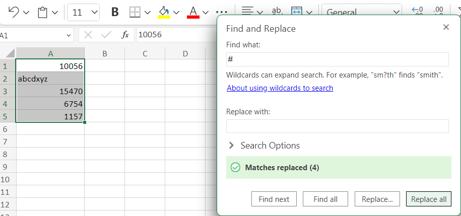

In the worksheet, the number of matches replaced is 4.

The Find and Replace Method are directly applied to the source data. Hence to get back the original data, press Ctrl+Z. It returns to the original data.

Example 3: What will result in case Sensitive Data using the Find and Replace Method?

In data, there occurs a repetition of numbers, characters, symbols, etc. The repeated data are present in both upper case and lower case. In this example, the working of the Find and Replace Method in Case Sensitive data is explained here.

Step 1: Enter the data in the worksheet, namely A1:A5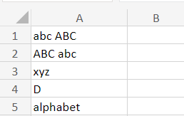

Step 2: Select the cell range from A1:A5, and Click Ctrl+H. The Find and Replace dialog box will open.

Step 4: The character 'abc' needs to be removed from the data. Hence in the FIND dialog box, enter the data as abc. The Replace dialog box should be left empty. Click Replace ALL.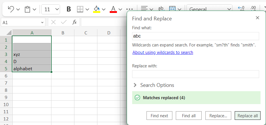

The given data contains both uppercase and lowercase ABC. The Find and Replace Method removes both the uppercase and lowercase characters. Hence Find and Replace Method is not a case-sensitive one.

Example 4: How to remove the specified characters using the formula?

Excel provides a formula method to remove specified characters in the data. The steps to be followed are,

Step 1: Enter the data in the worksheet, namely A1:A5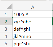

Step 2: Here, the symbol '^' needs to be removed from the given data. Select a new cell where the user needs to display the result, namely =VALUE (SUBSTITUTE (A1," ^ ",")).

Step 3: In the formula, A1 represents the cell that contains the data, and the symbol '^' is placed between double quotes and replaced with space.

Step 4: Press Enter. The result will be displayed in cell B1, where the specified symbol is removed using the formula. To get the result for the remaining data, drag the formula toward cell B5.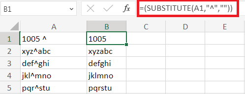

In the worksheet, the formula removes the specified data in the given data and displays the result in the selected cell.

Example 5: Remove the specified text in the given data using the formula.

Step 1: Enter the data in the worksheet, namely A1:A5

Step 2: The text Apple needs to be removed from the data. Select a new cell where the user needs to display the result, namely =VALUE (SUBSTITUTE (A1," APPLE ",")).

Step 3: In the formula, A1 represents the cell that contains the text, and 'APPLE' is placed between double quotes and replaced with space.

Step 4: Press Enter. The result will be displayed in cell B1, where the specified text is removed using the formula. To get the result for the remaining data, drag the formula toward cell B5.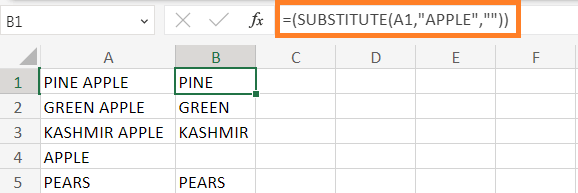

In the worksheet, the formula removes the specified data in the given data and displays the result in the selected cell.

Example 6: How to delete multiple characters in the given data?

Sometimes there is a need to remove multiple characters in a single data. To remove multiple characters, the formula to be used is as follows,

Step 1: Enter the data in the worksheet, namely A1:A5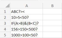

Step 2: Here, the character '?','>','<' needs to be removed from the given data. Select a new cell where the user needs to display the result, namely =SUBSTITUTE (SUBSTITUTE (SUBSTITUTE (A1,"? ","),">","),"<","")

Step 3: In the formula, A1 represents the cell containing the character and specified characters placed between double quotes and replaced with empty space.

Step 4: Press Enter. The result will be displayed in cell B1, where the specified characters are removed using the formula. To get the result for the remaining data, drag the formula toward cell B5.