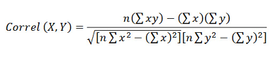
Excel CORREL function

In statistical analysis, many times, you are asked to find the relationship between two properties. However, there are various ways to achieve that, and one of them is by using the inbuilt CORREL function of Excel. In this tutorial, we will take a deeper look at the CORREL function.

What is Excel CORREL function?

The Excel CORREL function returns the correlation coefficient between 2 datasets. Correlation lies between -1 and 1, called negative correlation and positive correlation. It returns the correlation coefficient of array1 and array2. For example: as a baby grows older, the height or weight increases - implying that there is a relation between the age and height or age and weight, and with the increase in one, the other is also increasing, i.e., positive correlation.

CORREL or the correlation coefficient is very helpful to find out the relation between the two properties. If the specified array or reference parameter includes text/string, logical data, or an empty value, those data are ignored automatically. However, this function includes the cells that value zero in its calculation. The CORREL function is categorized under Excel statistical functions.

Though this works gives the same output as the Excel Pearson Function, with the only difference that in earlier versions of Excel (before Excel 2003), the Pearson function may throw some rounding errors. Therefore, if you are working with earlier Excel versions, it is advised to use CORREL as it will return a more efficient and accurate output. In later versions, both functions (CORREL and PEARSON) return the same outputs.

Note: If correlation coefficient r's value is close to +1, it shows a definite positive correlation, and if the value of r is near to -1, it indicates a definite negative correlation.

Syntax

Parameters

Array1 (required)- This parameter represents the first array for which you want to calculate the correlation value.

Array2 (required) - This parameter represents the second array for which you want to calculate the correlation value. It is a set of dependable variable.

Returns

The CORREL function returns the correlation coefficient of array1 and array2.

Things to Remember

• If the specified array or reference parameter holds text, logical values, or blank cells, the CORREL function ignores those values. However, this function includes the cells that value zero in its calculation.
• If both the parameters (array1 and array2) have a different number of data points, this function returns a #N/A error.
• If any one of the parameters is blank, or if s (the standard deviation) of their values is equal to zero, this function returns a #DIV/0! error.
• As much as the correlation coefficient r's value is close to +1, it shows a definite positive correlation. If the value of r is near -1, it indicates a definite negative correlation. A positive correlation indicates that if the values in one parameter increase, the values in the other array increase. In contrast, a negative correlation means that if the values in one parameter decrease, the values in the other array decrease.
• Below given is the equation for the CORREL value:
  
  Where, the values represent the sample.

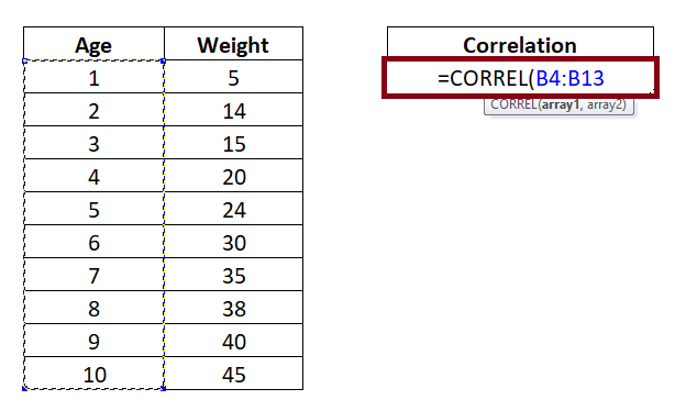
Examples

Example 1: Calculate correlation between Age and Weight for the following set of numbers.

To determine the correlation coefficient value between Age and Height, follow the below-given steps:

STEP 1: Add the helper column named "Correlation"

• Place your mouse cursor to the cell any and name the new column as "Correlation".

It will look similar to the below image: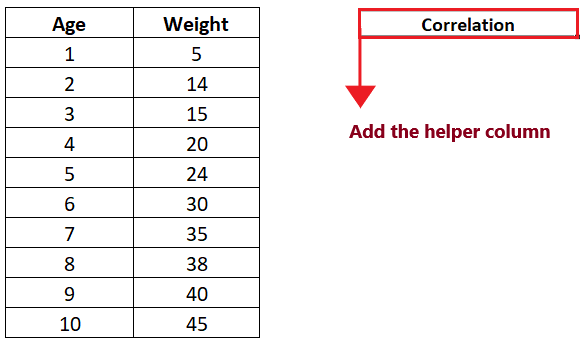

In this column, we will enter our CORREL formula. Though it's just for our reference if you want you can skip this step and directly move to STEP 2.

NOTE: Format the helper column and match it with the first column to make your Excel sheet more attractive.

STEP 2: Type the CORREL function

Move the cursor to the second row (cell reference E4) of your helper column and start typing the function = CORREL(

It will look similar to the below image: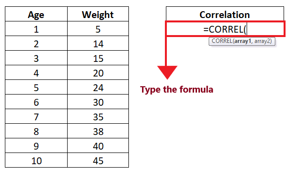

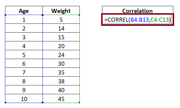
STEP 3: Insert the arguments, array1 and array2

• Insert the first parameter 'array1'. In this, we will enter the first array for which you want to calculate the correlation value. Here, we pass the array range reference of Age column data, i.e., B4: B13. The formula will be : =CORREL (B4:B13,)
  It will look similar to the below image:
  
• Insert the second parameter 'array2'. In this, the second array for which you want to calculate the correlation value. Here, we pass the array range reference of Weight column data, i.e., C4: C13. Therefore, the formula will be : =CORREL(B4:B13, C4:C13 )
  It will look similar to the below image:
  

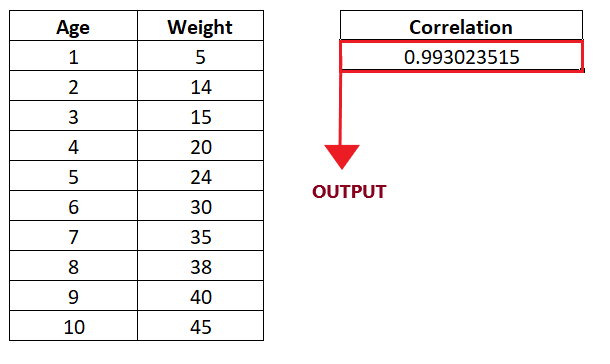
STEP 4: DATEVALUE will return the result

• Once done, press the enter key to fetch the output.
• The CORREL function will analyze both the data of array1 and array2 and will return the correlation coefficient between 2 datasets. In our case, it has returned a correlation value of 0.993023515.
  It will look similar to the below image:
  

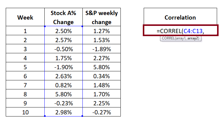
Example 2: In this example, we are given the data set of weekly changes for a stock A in column C and S&P weekly change in column c (refer to the below table). Based on these data values calculate the correlation coefficient of both the data using the CORREL formula in excel.

To determine the correlation coefficient value between the two data set, follow the below-given steps:

STEP 1: Add the helper column named "Correlation"

• Place your mouse cursor to the cell any and name the new column as "Correlation".

It will look similar to the below image: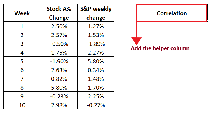

In this column, we will enter our CORREL formula. Though it's just for our reference if you want you can skip this step and directly move to STEP 2.

NOTE: Format the helper column and match it with the first column to make your Excel sheet more attractive.

STEP 2: Type the CORREL function

Move the cursor to the second row (cell reference c4) of your helper column and start typing the function = CORREL(

It will look similar to the below image: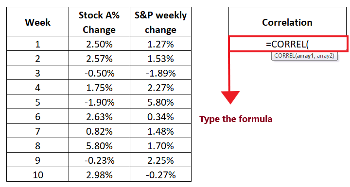

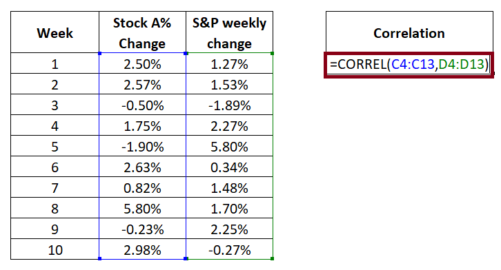
STEP 3: Insert the arguments, array1 and array2

• Insert the first parameter 'array1'. In this, we will enter the first array for which you want to calculate the correlation value. Here, we pass the array range reference of "Stock A% change" column's data, i.e., C4: C13. The formula will be : =CORREL (C4:C13,)
  It will look similar to the below image:
  
• Insert the second parameter 'array2'. In this, the second array for which you want to calculate the correlation value. Here, we pass the array range reference of "S&P weekly change" column's data, i.e., D4: D13. Therefore, the formula will become: =CORREL (C4:C13, D4: D13)
  It will look similar to the below image:
  

STEP 4: DATEVALUE will return the result

Once done press the enter key to fetch the output.

The CORREL function will analyze both the data of array1 and array2 and will return the correlation coefficient between 2 datasets. In our case it has returned a correlation value -0.309639228.

It will look similar to the below image: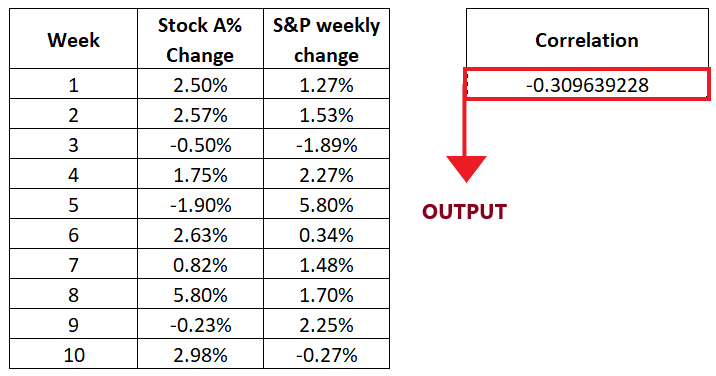

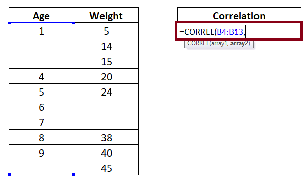
Example 3: In the below table, we have different height for both the data columns. Let's see what happens if you calculate the correlation between Age and Height for the following set of numbers.

To determine the correlation coefficient value between Age and Height, follow the below-given steps:

STEP 1: Add the helper column named "Correlation"

• Place your mouse cursor to the cell any and name the new column as "Correlation".

It will look similar to the below image: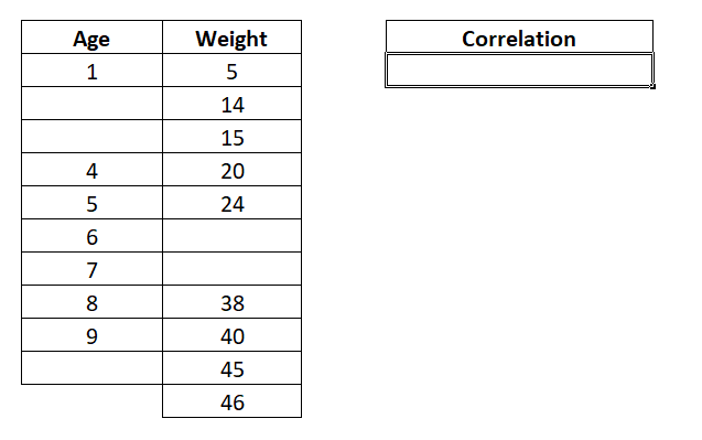

STEP 2: Type the CORREL function

Move the cursor to the second row (cell reference E4) of your helper column and start typing the function = CORREL(

It will look similar to the below image: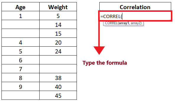

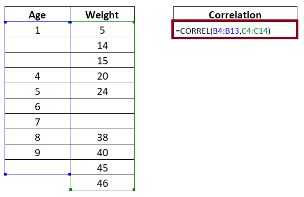
STEP 3: Insert the arguments, array1 and array2

• Insert the first parameter 'array1'. In this, we will enter the first array for which you want to calculate the correlation value. Here, we pass the array range reference of Age column data, i.e., B4: B13. The formula will be : =CORREL (B4:B13,)
  It will look similar to the below image:
  
• Insert the second parameter 'array2'. In this, the second array for which you want to calculate the correlation value. Here, we pass the array range reference of Weight column data, i.e., C4: C13. Therefore, the formula will become: =CORREL(B4:B13, C4:C13 )
  It will look similar to the below image:
  

STEP 4: DATEVALUE will return the result

• Once done press the enter key to fetch the output.
• The CORREL function will analyze both array1 and array2 and it will return the #N/A error. This error occurs because array1 and array2 are of different heights.

Refer to the below image for the output: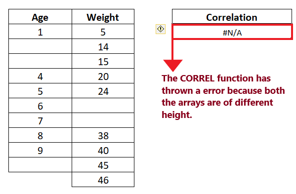

NOTE: The CORREL functions Correlation coefficient value only if both array1 and array2 are of the same length.

Correl Function Errors

While working with the CORREL function, if you get an error, this could likely be because of the following reasons:

• #N/A - This error occurs if the reference arrays (Array1 and Array2) are of different lengths.
• #DIV/0! - This error occurs if any one of the reference arrays is blank or if s (the standard deviation) of their values is equal to zero.