Excel Sort by Color

Excel provides loads of features when it comes to Sorting, and one such option is to Sort the Excel data by colour. Yes, Microsoft gives you the option to sort the content of the cells either manually coloured or conditionally coloured by their colour.

With the advanced sorting feature, we can easily position the cells containing a particular at the start or end of the specified list. For instance, you can place all your cell data containing blue at the top while the cells carrying red can be kept at the bottom.

Isn't that interesting? In this tutorial we will cover the following sort by colour topics wherein we will learn the exact steps to do this:

1. Sorting data with single colour
2. Sorting data with multiple colours
3. Sorting data based on Font colour
4. Sorting based on Conditional Formatting Icons
5. Sorting without losing the original order of the Data

Let's get started!

Sorting data with single colour

Sorting by a cell's background colour is very easy. If your dataset contains only a single colour, you can quickly sort it in any order based on the colour.

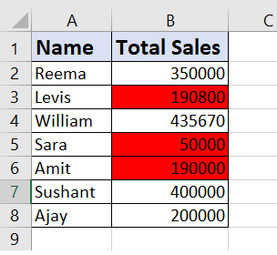
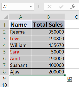
Here, we are given the following dataset where all the candidates who have achieved their sales target (amount < 200000 INR) are highlighted in red. Let's sort the cells and out the cells marked with red font colour at the top of the list.

Below given are the steps to sort the cells in terms of their colour:

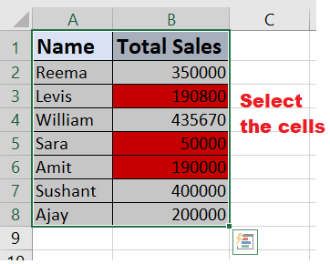
1. Select the range of cells that you want to sort. For instance, in our case we have selected the entire dataset i.e., A1:B8.
   
2. Go to the Data tab from Excel ribbon toolbar. Click on the 'Sort' option from the Sort & Filter section. It will open the Sort dialog window.
   
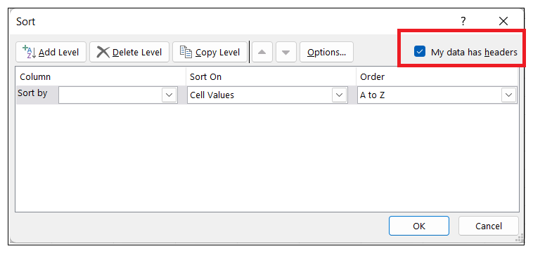
3. In the window, always ensure the you have selected the 'My Data has headers' option. In case the selected range doesn't contains headers, you can uncheck this option.
   
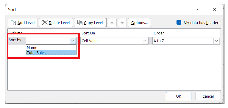
4. The next step is to click the 'Sort By' drop-down. From the resulting options, select the 'Achieved sales' column. This column represents the data based on which the sorting will be done.
   
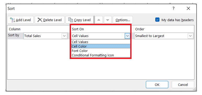
5. Go to the 'Sort On' drop-down option, and click on Cell Colour. As soon as you choose this option, you will notice two more drop down will appear within the same window.
   
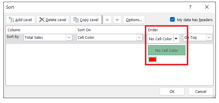
6. Click on the 'Order' drop-down, and it will open a window from where we can select the colour to sort the data. In our case, there is just one colour; therefore, it will only display one colour, i.e., red.
   
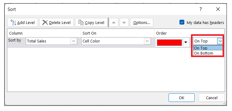
7. In the second drop-down in Order, select the On-top option. It asks you to specify whether you want to place the coloured dataset at the top or the bottom of the selected list. Since we want to align it at the top, we have selected the top option.
   
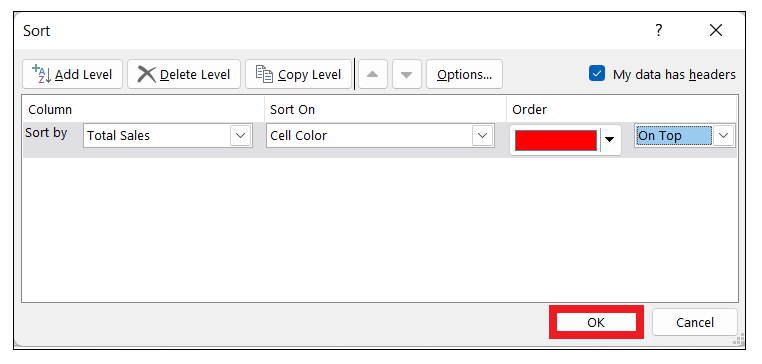
8. Once all the above steps are done, click on the OK button.
   

You will get the following output. As a result, you will notice the cells with blue colour are positioned at the top, whereas the rest of the cells remain as it is.

Note: Sorting based on colour only rearranges the cells and only brings together all the cells that are present in the same colour. It doesn't tamper with the arrangement of others to bring together all the cells of the same colour together.

Sorting data with multiple colours

In the above example, we only had cells with one colour that needed to be sorted. We can use the same methodology to sort when you have cells with multiple colours.

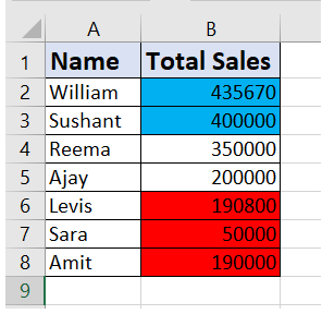
Let's suppose we are given a dataset wherein the candidates who have achieved their sales target (total sales >= 400000 INR) are marked with blue, and the candidates whose total sales are below 200000 INR are marked with red.

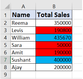
Question: The cells with blue should be at the top, those with red should be placed at the bottom of the list, and those without any colour should be in the middle.

Below given are the steps to sort the cells in different order on the basis of multiple colour:

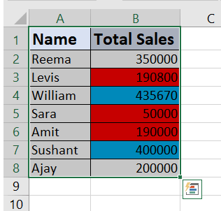
Step 1: Select the dataset

Select the range of cells that you want to sort. For instance, in our case we have selected the entire dataset i.e., A1:B8.

Step 2: Sort the data cells with red font colour

1. Go to the Data tab from Excel ribbon toolbar. Click on the 'Sort' option.
   
2. If your data contains header make sure that you have selected the 'My Data has headers' option.
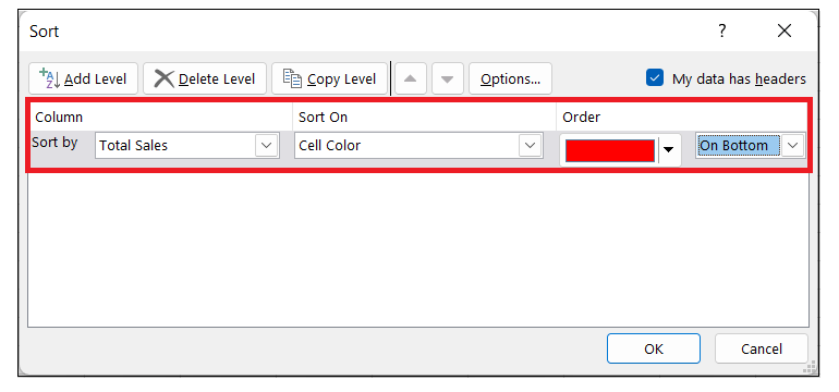
3. The next step is to click the 'Sort By' drop-down. From the resulting options, select the 'Total sales' column. This column represents the data based on which the sorting will be done.
4. Go to the 'Sort On' drop-down option, and click on Cell Colour.
5. Click on the 'Order' drop-down, and select the colour based on which you want to sort the selected data. It will show all the colour present in the selected data. In our case, there are just two colours, but we will choose the red one.
6. In the second drop-down in Order, select the On-bottom option.

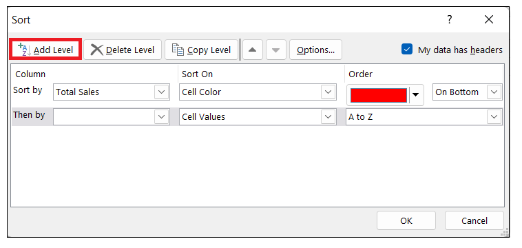
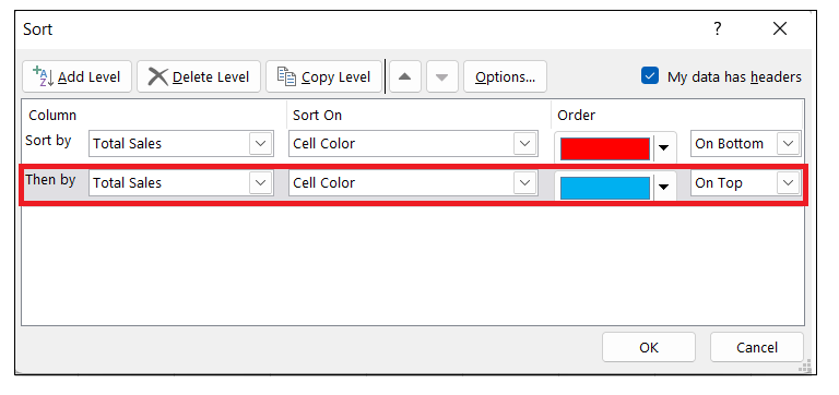
Step 3: Sort the data cells with blue font colour

1. Since we want to add other condition of sorting as well therefore, we will click on Add Level button. Clicking this option will add another colour sort options.
   
2. Go to 'Then-by' dropdown window. Select Marks.
3. From the 'Sort On' drop-down option, select the second Cell Colour.
4. From the 'Order' drop-down, we will choose select the second colour to sort the data. It will display all the colours in the dropdown that are present in the selected dataset. Select the blue colour.
5. In the second drop-down in Order, select On-Bottom.

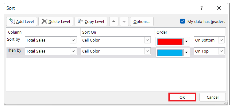
Step 4: Click on OK

Once done, click on the OK button. You will get the following output.

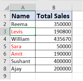
To your surprise the cells with blue colour are positioned at the top whereas the one if red are positioned at the bottom as shown below.

Sorting data based on Font colour

Another overwhelming Microsoft feature in Excel is that it enables users to sort by font colour in the cells. While this is not a common practice, this is still something many Microsoft Excel users do.

In the example below, we are given a dataset where the names that have achieved a sales target of less than 200000 INR are marked with red font.

Question: We have to sort the above dataset, where the cells whose text is with red font colour need to be grouped at the top of the list.

Below given are the steps to sort the cells in a different order based on data font colours:

1. Select the range of cells that you want to sort. For instance, in our case we have selected the entire dataset i.e., A1:B8.
   
2. Go to the Data tab from Excel ribbon toolbar. Click on the 'Sort' option. It will open the Sort dialog window.
   
3. In the window, always ensure the you have selected the 'My Data has headers' option. In case the selected range doesn't contains headers, you can uncheck this option.
   
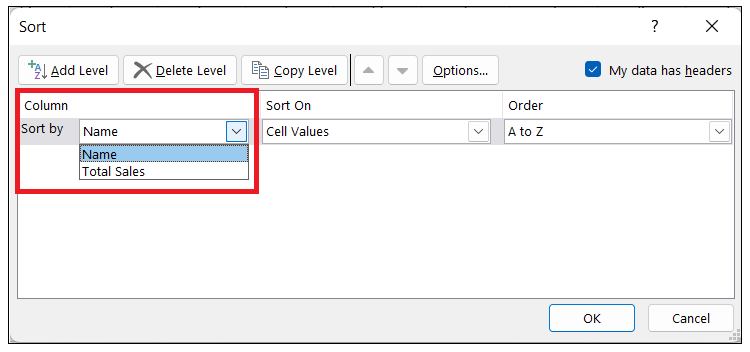
4. The next step is to click the 'Sort By' drop-down. From the resulting options, select the 'Name' column. This column represents the data based on which the sorting will be done.
   
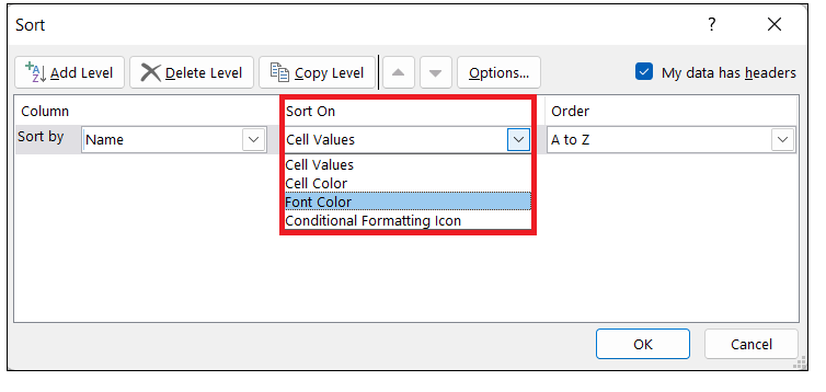
5. Click on the 'Sort On' option. From the resulting drop-down choose the Font colour option.
   
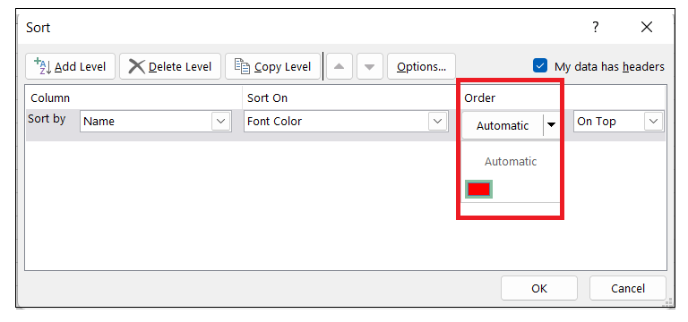
6. In the 'Order' drop-down, select the colour based on which you want to sort the data. Since there is only one colour in our dataset, it only shows one colour (red).
   
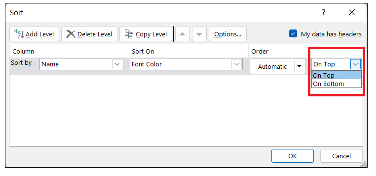
7. In the second drop-down in Order, select On-top. This is the place where you specify whether you want all the coloured cells at the top of the dataset or at the bottom.
   
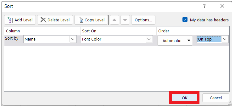
8. Once you are done with all the steps, click on the OK button.
   

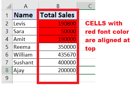
You will get the following output.

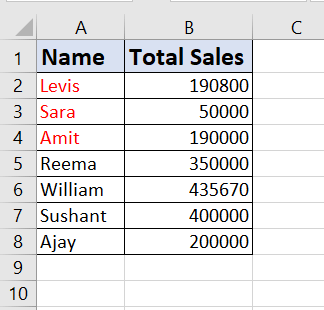
You will notice all the names with red font colour are aligned at the top of the selected list.

Sort Based on Conditional Formatting Icons

Conditional formatting is a Excel feature that helps its users to creative visual icons in their worksheet. It makes your data or your dataset look more professional and easier to read.

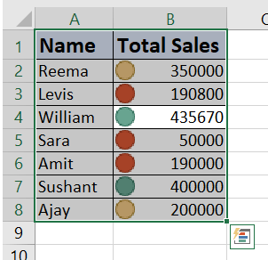
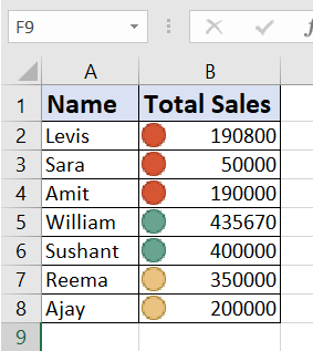
In the following example, we have used conditional formatting icons where the red circles are put in front of the data whose sales value is less than 200000 INR. The orange icon is set to the one whose sales value is less than 400000 INR and greater than 200000 INR, and the blue icon to the one whose value is greater or equal to 400000 INR.

Below given are the steps to sort the cells in different order on the basis of conditional formatting icons:

STEP 1: Select the cells and click on SORT option

1. Select the range of cells that you want to sort. entire dataset. For instance, in our case we have selected the cells A1:B8.
   
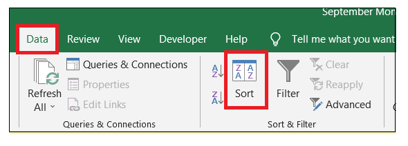
2. Go to the Data tab from Excel ribbon toolbar. Click on the 'Sort' option. It will open the Sort dialog window.
   

STEP 2: SORT the red icon at the top of the list

1. Since the selected data contains header, therefore we check the 'My Data has headers' option from the window.
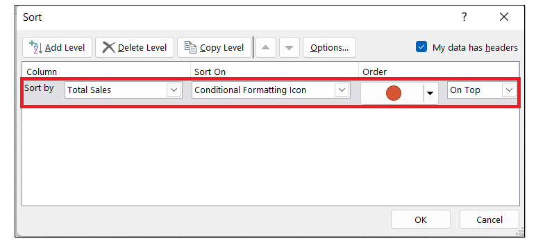
2. Go to the 'Sort By' drop-down option and choose the 'Total sales' column. It contains the conditional formatting icon based on which we want to sort the data.
3. Click on the 'Sort On' drop down window, from the listed options select the 'Conditional Formatting Icon'.
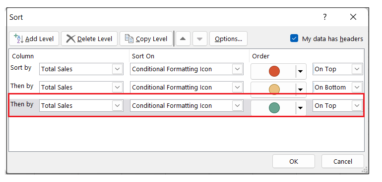
4. Go to the 'Order' drop-down, select the icon colour based on which you want to sort the data. Since our column contains three different icons so it will show all the icons. We will choose the red icon.
5. From the second drop-down in Order, we will choose the On-top option.

STEP 3: SORT the Green icon at the middle of the list

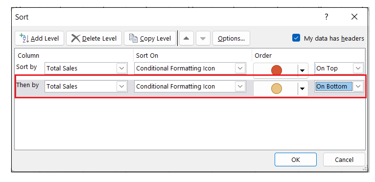
1. To add another condition, we will click on Add Level button. Using this option, we can easily add another colour sort option.
2. Click on the to the 'Then by' drop-down option, select the 'Total Sales' column.
3. Click on the 'Sort On' drop down window, from the listed options select the 'Conditional Formatting Icon'.
4. Go to the 'Order' drop-down, select the icon colour based on which you want to sort the data. We will choose the orange icon.
5. From the second drop-down in Order, we will choose the On-bottom option.

STEP 4: SORT the red icon at the bottom of the list

1. Since we have to add another sorting option, therefore, again we will click on Add Level button.

NOTE: In case, you want to sort fourth conditional icon we will again click on this icon.

2. Click on the to the 'Then by' drop-down ' option, select the 'Total Sales' column.
3. Click on the 'Sort On' drop down window, from the listed options select the 'Conditional Formatting Icon'.
4. Go to the 'Order' drop-down, select the icon colour based on which you want to sort the data. We will choose the red icon.
5. From the second drop-down in Order, we will choose the On-Top option.

STEP 5: Click on OK to fetch the output

1. Once done, you can click on the OK button.
2. As the result, once the above steps are complete you will have the following result where all the similar icons are sorted and put together.

Note: In the case of multiple sorting, the sequence of the sorting order will be followed precisely as it has in the sorting window. In the above example, as you can see, we have positioned the red icon set at the top, the orange in the middle and the green in the middle. Therefore, the output has also followed the same sequencing order.

Sorting without losing the original order of the Data

Once the sorting is done, you will lose the original data since all the changes are made in the same place replacing the original data. But if you want to keep safe your original data as well, always make sure to copy the data and paste it in another worksheet and then apply the sorting on the copied data.

OR

Another quick method to ensure that you can retrieve your original data is to add a helper column with row numbers. Follow the below steps:

1. Add a helper column next to the last column. (refer to the below screenshot)
   
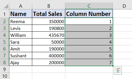
2. Once you have inserted the helper column in your worksheet, perform the sorting operation.
3. In case you want to put back your original data afterwards, you can easily sort this data using the serial numbers of this helper column.