How to add prefix in Excel?Adding a prefix is not so needy thing to do in Excel. It might sometimes require to add a prefix before the text or string. A prefix can be any text or string type of data you want to insert before any data inside the Excel cell. For example, Mr. string before each name of the mail person in an Excel sheet or add Dr. before each person name whose profession is doctor. Hence, the prefix takes place in this way. When the Excel users add a string at the beginning of the cell is called prefix. When a text string is added at the end of the string is called suffix. Why to add prefix?A prefix can be manually added to any cell data. But when you need to add the same prefix to multiple cells data, you can add it by using another method. Because adding the prefix to multiple cells one by one will take too much time. In the same way, suffix takes place. Suppose you are working with a large set of data in an Excel sheet and want to add prefix or suffix. Manually adding any suffix or prefix to a large dataset take too much time and will become hectic. Concatenation function or & operator can be used for this purpose. Perhaps you will find it easy and fast to add a prefix in any data stored in an Excel sheet. Ways to add prefixThere are two ways to add a prefix to any data in an Excel sheet.
Add prefix using CONCATENATE functionCONCATENATE() is a function offered by MS Excel that you can use to add prefix or suffix to your Excel data. Basically, it is used for the concatenation operation. Make use of this function to add the prefix to the data. For example, we will add Dr. as a prefix to the column A data Syntax for CONCATENATE() function Both string parameters are passed to be merged together in a single string. Example 1 We have the data of doctors for this example that will show the method to add a prefix in data. We will add Dr. as a prefix to their names in a range of cells by using CONCATENATE() formula. We have prepared this data on which we will show you the implementation of CONCATENATE() function. 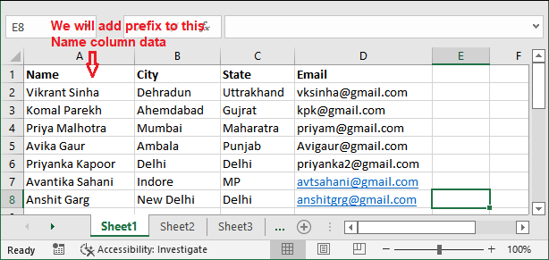
Let us follow the steps for it, same as below - Step 1: Firstly, add a new column next to the Name column. 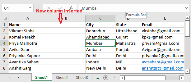
Step 2: In this new column, write the following formula with the prefix string you want to add with the name. =CONCATENATE("Dr.", A2) 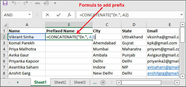
Step 3: Press the Enter key on your keyboard and see the concatenated string. Both strings are successfully merged. 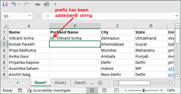
Similarly, we can do with the other cells. As we have to put the Dr. as a prefix to each cell in column A. Step 4: So, go to the B2 cell and take the mouse cursor at the bottom right corner. A + sign will enable near to this. Drag this + sign in the below cells to copy the formula for them. 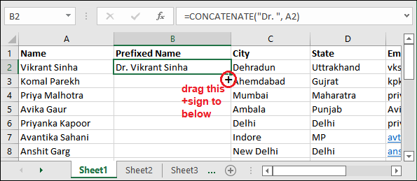
Step 5: See that a prefix string Dr. is placed before each name till when we have copied the formula. 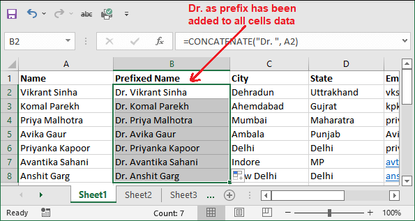
This process makes it easy for the users to add a prefix before the data in different cells in MS Excel. Add prefix using & operatorAnother method to perform the concatenation operation on Excel data is using & operator. This will also help the users to concatenate the string. Ampersand & is an operator that can be used in Excel to concatenate the string. Syntax to add prefix using & operator Here, we have the previously prepared where column A contains the name of doctors in this Excel sheet. 
We will use the & operator to add a prefix in the column A data. Let us follow the steps for it, same as below - Step 1: Add a new column next to it that will contain the resultant data after adding a prefix to doctors names. 
Step 2: Now, write the following formula in the B2 cell with the prefix string you want to add with the name. ="Dr. " &A2 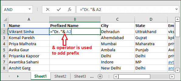
It will concatenate the A2 cell string with the prefix string you passed in the formula. Step 3: Press the Enter key on your keyboard and see the concatenated string. Both strings are successfully merged. 
In the same way, we can do more data. This one is the advantage of the & operator that we can concatenate more than one string at once using & operator. Step 4: So, go to the B2 cell and take the mouse cursor at the bottom right corner. A + sign will enable near to this. Drag this + sign in the below cells to copy the formula for them. 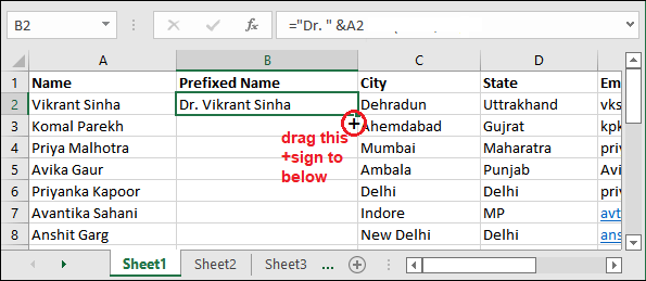
Step 5: See that a prefix string Dr. is placed before each name till when we have copied the formula. 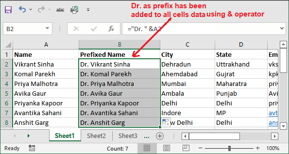
You have seen that the same formula is copied to each cell. It saves the time of users to manually add the same prefix to each cell. "Remember it will not help you when you need to add different prefix to each cell data." Add prefix and suffix to stringAs we previously told you, we could concatenate more than one string using & operator. We will elaborate you an example in which we will add both prefix and suffix to a previously defined string. So, you will learn to merge more than one string with the help of single formula. Let us follow the steps for it, same as below - Step 1: We have prepared the following data to implement and add the prefix or suffix to the given data. We will store the result in column B after adding prefix and suffix to the data. 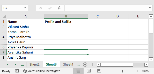
Step 2: Now, write the following formula in the B2 cell with the prefix string you want to add with the name. ="Mr. " &A2& ", PHD Professor" 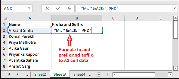
Here, Mr. is prefix and PHD Professor is the suffix. It will concatenate the A2 cell string with the prefix string you passed in the formula. Step 3: Press the Enter key on your keyboard and see the concatenated string. See that the prefix and suffix are added to the string. 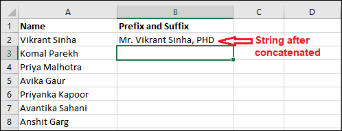
Step 4: Concatenate another cell data by using the below formula in B3 cell. ="Mr. " &A3& ", PHD Professor " 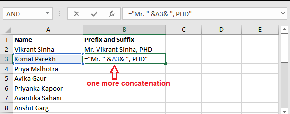
Step 5: Press the Enter key and get the concatenated data that has been returned after merging the strings together. 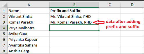
You can drag the formula as we done in the above methods to copy the same formula and implement it to the below cells. Add prefix in batchSometimes the Excel users need to the same prefix on more than one cell at a time. As we already had discussed the way to add prefix or suffix using CONCATENATE() function & operator. We have another method for adding the prefix and suffix to the Excel data. You will find this method easy than the above ones. Even you do not need to put any formula or use any operator for this. You just need to select and apply some steps to add the prefix. Advantage of using this method:
Steps to add the prefix in batchLet us see how we can add the prefix to multiple cells without using a single formula to it. Step 1: We have employee id in column A which is numeric data. We want to add prefixes and make them alphanumeric by adding a string EMP to them. Step 2: Select the cells in bulk before which you want to add the prefix to it and press the Ctrl+1 key. Step 3: In the Number tab, move to the Custom tab in the left sidebar. Step 4: Now, write the prefix you want to add inside the Type field before the General. Then, click OK in the last. We have added EMP here. Step 5: You will see the prefix is added to the selected data. You have seen that we have not used any formula to add the prefix to it. Remember, one most important thing is that it does not enter actual content. It just only changes the format of the cells you have selected. Add prefix based on conditionIn all the above examples, we have used only string type of data. But do not confuse or worry that you cannot merge another type of data. You can also merge numeric data. We will now show you to concatenate the numeric data. For example, country code before the mobile number (+91 for Indian mobile number). We will also try to make it conditional based. Like, where the country is India, +91 will be added as a prefix string to the mobile number in each record. It will be a little complicated before the above methods. We can achieve this by combining the custom number format with conditional formatting. We have to implement conditional formatting for this. Let us implement and see how it will be done. Here, column A contains the name of doctor in this Excel sheet. Create a dropdown list using validation ruleWe will create a dropdown list having a list of countries. Based on the selection of country, a country code is added as a prefix to the mobile number. Step 1: We have taken some mobile numbers in a column and a country column to take the input from users. 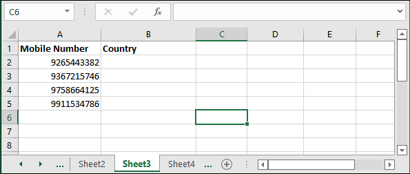
Step 2: So, create the dropdown list for column B, select column B from the header and move to the Data tab. 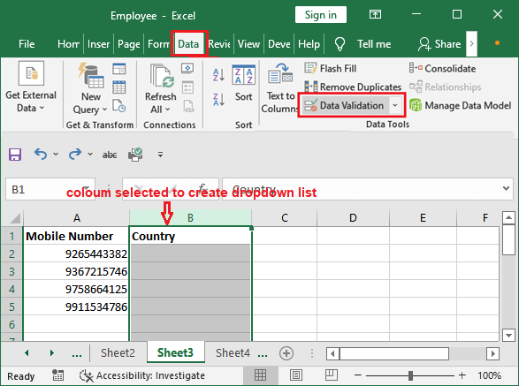
Step 3: Here, click the Data Validation inside the data Tools to create the dropdown list. 
The ropdown list comes under the Data validation category in MS Excel. Step 4: Now, Choose List inside the Allow field. Then, enter the names of countries, separate them by comma and click OK. 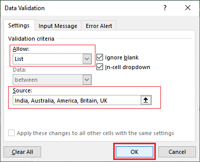
Step 5: A dropdown list of countries has been created for column B. 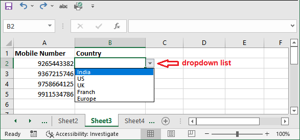
Implement the conditional formattingNow, we will apply conditional formatting to data. It means when the user selects one of the countries from the list, country code will be added as a prefix to the mobile number in its respective cell. Step 6: Select column A (it is our targeted column). And click the Conditional Formatting inside the Home tab. 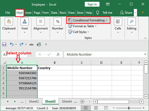
Step 7: Choose New Rule from the Conditional Formatting list. 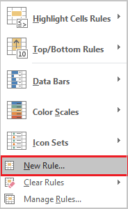
Step 8: Choose Use a formula to determine which cells to format for a rule type. Write the formula =B1="India" that will format the values when the formula will true. Click the Format to apply the formatting on data. 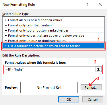
India is the country; we have added it inside the dropdown list in column B. Step 9: In this panel, switch to the Custom tab (inside Number tab in the header) and enter "(+91)" 0 in the Type field and then click OK. 
Step 10: Preview the formatting and click OK if everything is correct. The (+91) string will be added the same as like in the preview field. 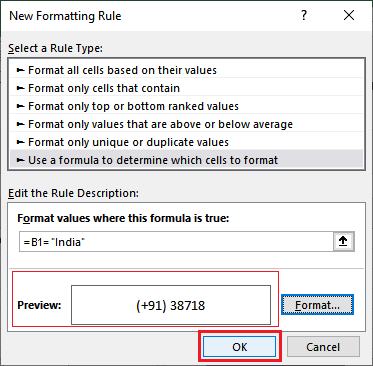
Step 11: Repeat step 6 to step 10 for the other countries with their country code of dropdown list you have created. We have also created conditional formatting at our end for other countries. You do it too. Recheck all the rules createdStep 12: Now, click Conditional Formatting Inside the Home tab and choose Manage Rules. Home > Conditional Formatting > Manage Rules 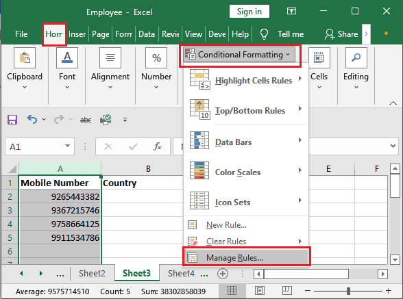
Keep selecting column A to see all the rules for this column. Step 13: All the rules you have created will display here. In case rules are not showing, choose This Worksheet inside the Show formatting rules for. We find everything fine here. So, we clicked the Apply button. 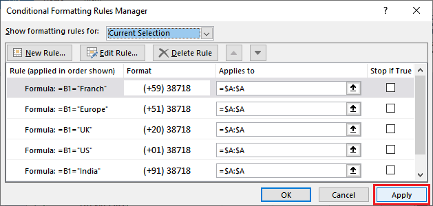
Here, you notice that the Applies to cell having correct data cells. So, we will change them. Also, if you made any mistake while creating the conditional formatting rule, you can edit from here by double-tapping on that rule. Step 14: Now, click OK to close the panel. 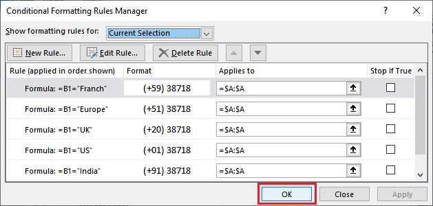
Step 15: When you choose a country from the dropdown list in column B, chosen country code will automatically place before the mobile number in the corresponding cell. 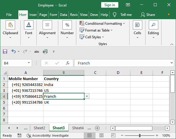
See in the above screenshot that we have selected different countries in column B and the different code is applied to the mobile number. This is the dynamic way to add the prefix to Excel data. In the similar manner, you can find other ways to add prefix by putting conditional formatting on a column. For example, on direct input in a column rather than a dropdown list input and it will reflect on another column data based on some condition. You do not need to all time create a dropdown list, you can directly put a condition on data. Let us understand with an example for this too. Example 2: Add prefix based on conditionWe have taken the names of some people that belong to certain qualifications or degrees. Based on their qualification, we will add a prefix to their names. For example, Dr. is added as a prefix to the name of the person whose qualification is PHD. For achieving this, we will use conditional formatting on the qualification column and format the name column data. This change will occur in the name field when the user will provide the value in qualification field. We will not create any dropdown list for this. You may find this method easier than the above one. Steps to add prefix based on condition Step 1: Select the Name column (it is our targeted column) and click the Conditional Formatting inside the Home tab. 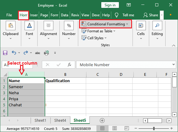
Step 2: Choose New Rule from the Conditional Formatting list. 
Step 3: Choose Use a formula to determine which cells to format for a rule type. Write the formula =B1="PHD" that will format the values when the formula will true. Click the Format to apply the formatting on data. 
Step 4: In this panel, switch to the Custom tab (inside Number tab in header) and enter "(Dr.)" 0 in the Type field and then click OK. 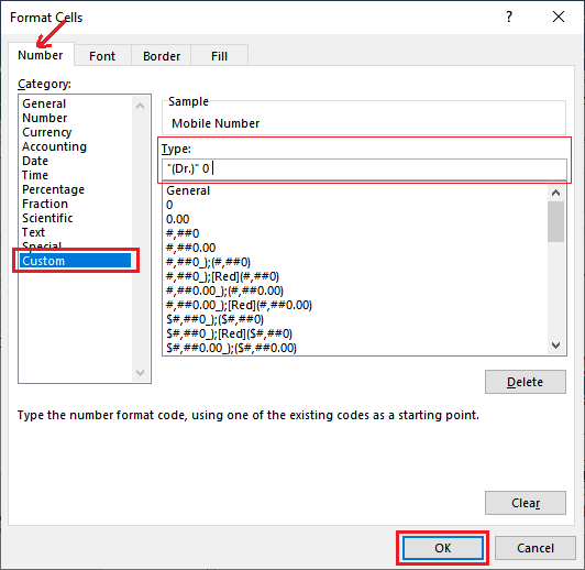
Step 5: Preview the formatting and click OK if everything is correct. The (Dr.) string will be added the same as like in the preview field. 
Step 6: Now, repeat step 1 to step 5 for the Engineering and use (Eng.) as a prefix. Recheck all the rules createdStep 6: Now, click Conditional Formatting Inside the Home tab and choose Manage Rules. Home > Conditional Formatting > Manage Rules 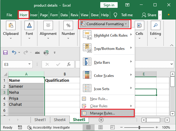
Keep selecting column A to see all the rules for this column. Step 7: All the rules you have created will display here. In case rules are not showing, choose This Worksheet inside the Show formatting rules for. We find everything fine here; click OK to close the panel. 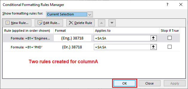
"If you had made any change, then first use Apply after that click OK." This will apply the changes to the updated data here. Step 8: Now, enter the data in the qualification column. If it meets with the condition, prefix you had set while created will place in the corresponding name cell. 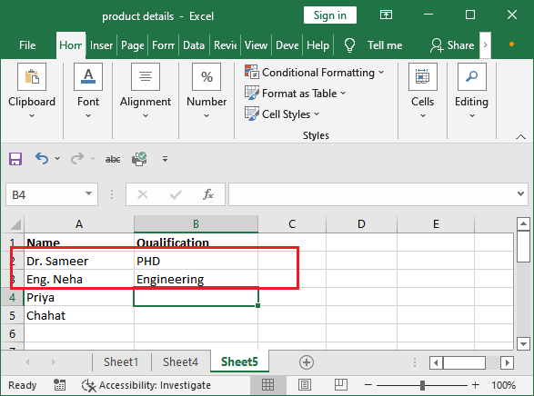
See in the above screenshot that we have selected different countries in column B and the different code is applied to the mobile number.
Next TopicShow formula in Excel
|
 For Videos Join Our Youtube Channel: Join Now
Feedback
- Send your Feedback to [email protected]
Help Others, Please Share


