Excel Rules Manager
We often use the Conditional Formatting tool in Microsoft Excel to highlight the cells in your working. The good part is Excel enables the users to apply two or more rules simultaneously. It even extends the functionality to control those rules as well as edit, delete, or duplicate. For that they introduced another section in conditional formatting named with 'Rules Manager'.
If you want to highlight the cell with unique data values and values greater than 200, you can need to apply two conditional formatting rules to the same set of cells in your Excel worksheet. With the Excel Rules Manager, you have an effortless way to check and manage all of your conditional formatting rules.
What is Excel Rule Manager?
"Excel Conditional Formatting Rules Manager gives you the freedom to view all conditional formats applied in the worksheet unlike the current selection or the rule created to highlight unique values. One can then insert a new rule, edit, and delete rules and can even rearrange the order of rules for the selected cells or worksheet"
The Excel Manage Rules option is listed in the Conditional Formatting menu, found in the 'Styles' group of the Home tab on the Excel ribbon. As soon you select this option, a secondary window pops up displaying the various rules applied to current selection, worksheet or various other sheets of the same workbook.
How to Open the Rules Manager in Excel?
Before opening the Conditional Formatting Rules Manager, make sure you open a specific worksheet and apply some rules to the numeric data. However, this option also allows the user to switch in between the sheets containing the conditional formatting rules within the same workbook.
Below given are the steps to quickly open the Top Rules Manager in your Excel worksheet:
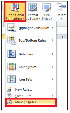
- Go to the Home tab of the Excel ribbon. Click on the Conditional Formatting drop-down arrow listed in the Excel' Styles' group.
-
It will open a window comprising the list of conditional formatting options; select the "Manage Rules".

-
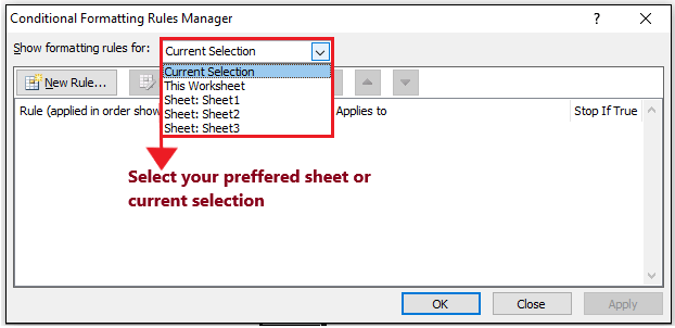
It will open the Conditional Formatting Rules Manager window (refer to the below image). From the 'Show Formatting rules for:' drop-down, select any sheet or the current worksheet for which you want to view the rules.

-
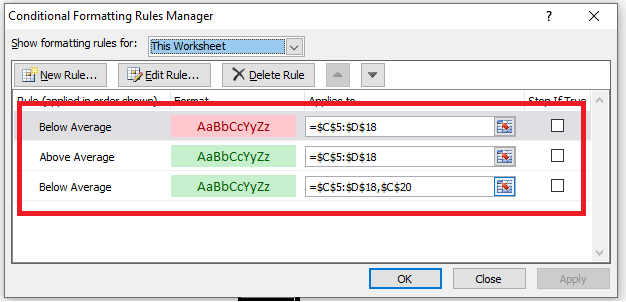
As soon as you select any sheet or the current selection, you will notice that the bottom panel of the window will display all the rules you applied for the selected sheet or range.

Manage Conditional Formatting Rules
Below given are the steps to quickly manage the rules applied in your Excel worksheet:
- Go to the Home tab of the Excel ribbon. Click on the Conditional Formatting drop-down arrow listed in the Excel' Styles' group.
-
It will open a window comprising the list of conditional formatting options; select the "Manage Rules".

-
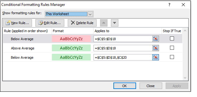
It will open the Conditional Formatting Rules Manager window (refer to the below image). From the 'Show Formatting rules for:' drop-down, we will select 'This worksheet'. All the rules applied on that worksheet will be displayed in the bottom panel.

-
On the top of the Rules Manager, you will find various rule manager actions that you can take. Select an action and, click "Apply".

- At last click on "OK" button to apply the changes in your worksheet.
Create a New Rule
Although the pre-defined rules are extremely helpful but in many cases those don't fulfill your requirement. Excel allows you to create a new rule so as you can customize your worksheet as per your own needs.
Below given are the steps to create a new rule using the conditional formatting Ruler Manager:
- Go to the Home tab of the Excel ribbon. Click on the Conditional Formatting drop-down arrow listed in the Excel' Styles' group.
-
It will open a window comprising the list of conditional formatting options; select the "Manage Rules".

-
It will open the Conditional Formatting Rules Manager window (refer to the below image). From the 'Show Formatting rules for:' drop-down, we will select 'This worksheet'. All the rules applied on that worksheet will be displayed in the bottom panel.

-
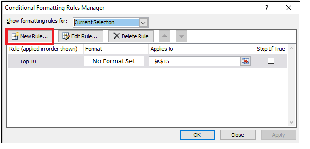
Click on "New Rule" option listed below the 'Show formatting rules for:"

-
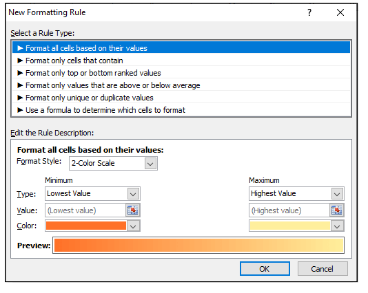
It will open a secondary window from where you can select any set of rules or can customize your own. Click on OK.

Change the Precedence of Conditional Formatting Rules
When there you have multiple rules in your excel data, it is possible that two or more rules could apply simultaneously to a single cell. To avoid ambiguity, you may need to define the order of the rules applied to the cell. The rule which has top precedence will be given priority.
Here's an example: Let's suppose you want to highlight the values based on their ranking. You have created a few rules to highlight a cell that contains values below average and lies in the bottom 30 percent. But the below-average cell values are your top concern. In such cases, you can manage precedence of the rule so that if the below-average rule applies to those cells, it will stop there and not highlight those in the bottom 30 percent.
Following are the steps to change the order of conditional formatting rule in Excel worksheet using Rule Manager:
- Click a cell in the range with multiple conditional formatting rules.
- Go to the Home tab of the Excel ribbon. Click on the Conditional Formatting drop-down arrow listed in the Excel' Styles' group.
-
It will open a window comprising the list of conditional formatting options; select the "Manage Rules".

-
It will open the Conditional Formatting Rules Manager window (refer to the below image). From the 'Show Formatting rules for:' drop-down, we will select 'This worksheet'. All the rules applied on that worksheet will be displayed in the bottom panel.

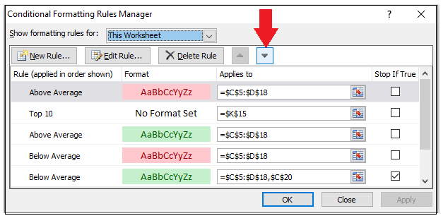
- In front of every rule you will notice a check box indicating the Stop If True setting.
- Select the rule for which you wish to change the order.
-
To move the rule up in order, click on Move Up. To move the rule down in order, click Move Down.

- Click OK.
That it! The conditional formatting rules are applied in your worksheet as per the specified precedence.
Delete a Rule
Sometimes you create a new rule that is no longer of any use. In such case you can delete the rule as well.
Following are the steps to delete a Rule in Excel worksheet using Conditional Formatting Rule Manager:
- Go to the Home tab of the Excel ribbon. Click on the Conditional Formatting drop-down arrow listed in the Excel' Styles' group.
-
It will open a window comprising the list of conditional formatting options; select the "Manage Rules".

-
It will open the Conditional Formatting Rules Manager window (refer to the below image). From the 'Show Formatting rules for:' drop-down, we will select 'This worksheet'. All the rules applied on that worksheet will be displayed in the bottom panel.

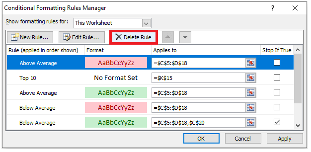
- If there are multiple rules so just select the one that you wish to delete.
-
Click on "Delete Rule" option listed below the 'Show formatting rules for:"

- Excel does not confirm the delete action. Once you click on delete the conditional formatting rule is deleted forever.
Example 1 - Using Excel Conditional Formatting Rules Manager, highlight the cells with two non-numeric values with different colors.
The below-given table has three fields name of the student, marks, and achieved grades. Highlight the grades column data with color such as "A" grade with Green color and "B" grade with red color.
| Name of the student |
Score |
Grade |
| Rahul |
657 |
C |
| Varun |
890 |
B |
| Himanshu |
543 |
C |
| Tina |
678 |
C |
| Jackeline |
980 |
A |
| Soheir |
800 |
B |
| Mohammed |
500 |
C |
Solution: Below given are the detailed steps to highlight the grades with two different colors:
STEP-1 Select the range of cells
Select the entire range of cells or the array, in which you wish to highlight the values. In our case, we have selected the cells from E5 to E11.
Refer to the below image:

Step 2: Type the New Rule
-
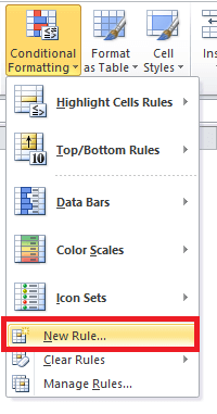
Go to the Home tab of the Excel ribbon. Click on the Conditional Formatting -> New Rule.

-
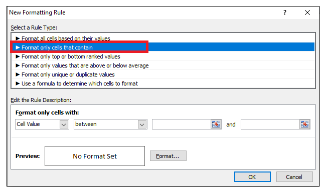
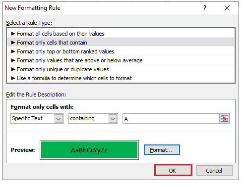
The 'New Formatting Rule' window will appear. From the first drop-down window select the rule type "Format only cells that contain"

- You will notice the data of bottom panel will change automatically as soon you select a rule type.
-
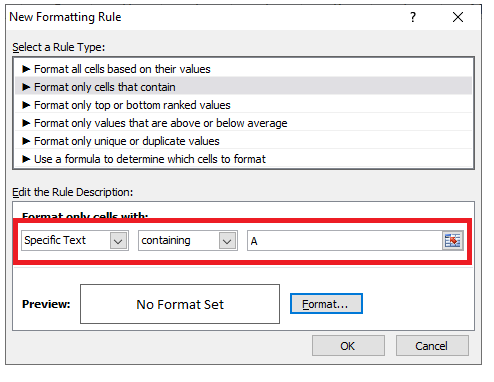
In the first drop down (cell value), select "Specific Text". In the second drop down window select "Containing". In the third textbox type "A".

-
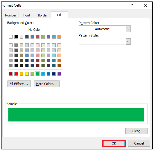
Click on the Format option located at the bottom. The format cells window will appear. From there select the green color in the Fill tab and click on OK.

-
The same color will be shown in the preview box. Click on Ok.

Step 3: Select Conditional Formatting Manage Rules
- Go to the Home tab of the Excel ribbon. Click on the Conditional Formatting drop-down arrow listed in the Excel' Styles' group.
-
It will open a window comprising the list of conditional formatting options; select the "Manage Rules".

-
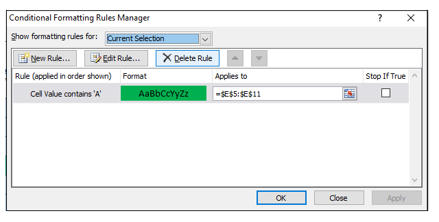
It will open the Conditional Formatting Rules Manager window (refer to the below image). From the 'Show Formatting rules for:' drop-down, we will select 'This worksheet'. All the rules applied on that worksheet will be displayed in the bottom panel.

Step 4: Using the Rule Manager Create a new Rule
-
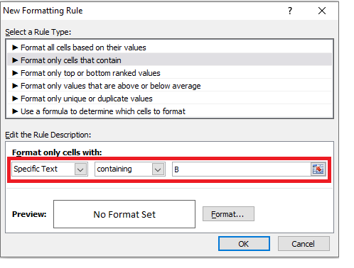
The 'New Formatting Rule' window will appear. From the first drop-down window select the rule type "Format only cells that contain"

- You will notice the data of bottom panel will change automatically as soon you select a rule type.
-
In the first drop down (cell value), select "Specific Text". In the second drop down window select "Containing". In the third textbox type "B".

-
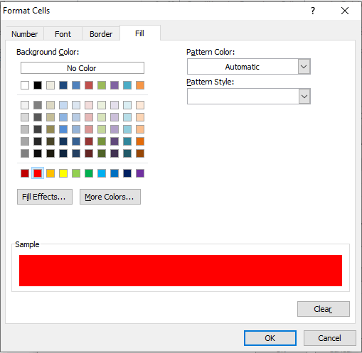
Click on the Format option located at the bottom. The format cells window will appear. From there select the Red color in the Fill tab and click on OK.

- The same color will be shown in the preview box. Click on Ok.
Step-4 Cells with grade A and B are highlighted
As a result you will notice all the cells containing value A are highlighted with green color and the cells containing value B are highlighted with red color.
Look out at the below figure for the resulting output.

| 

 For Videos Join Our Youtube Channel: Join Now


