Excel FV Function

Future planning is essential for making your personal and corporate finances. It is one of the most significant factors of success to understand the future perspective and growth of today's investment. To make this step easy, Excel has provided an inbuilt function known as FV (stands for future value).

In this tutorial, we will cover the definition, syntax, and the steps to build correct FV formula for a series of cash flows, various examples, and more!

What is FV function?

The Excel FV function tells the future worth of constant payments at a fixed interest rate (fixed value). It operates for both types of payments, whether a series of periodic payments or a single lump-sum payment.

The FV function is categorized under Excel Financial functions. This function is used to return the future value of an investment for a constant rate of interest. The future value (FV) is one of the prime elements that help in various financial modeling and benefits in financial planning. In other words, FV defines how much specific money or asset will rise or grow in the future if it is invested for a specific time.

Generally, the Future Value is calculated based on a predicted growth rate or rate of return. Determining a future value is quite easy when the money is deposited in a saving account with a fixed interest rate such as FD (Fixed deposit, RD, etc.). Though some investments have a volatile rate of return, and their interest rate also fluctuates, such as stocks, bonds, or other securities. These kinds of investments are hard to calculate accurately. Fortunately, Microsoft Excel has introduced a special function that does all the necessary calculation for you based on your given parameters.

The function was introduced with Excel 2007 and since then has been available in all versions, including Excel 2010, Excel 2013, Excel 2016, Excel 2017, and Excel 365.

Syntax

of that number.

Parameters

Rate (required)- This argument represents the rate of interest per period. If you pay once a year, supply an annual interest rate; if you pay the amount each month, then you should supply a monthly interest rate, and so on.

Nper (required) - This argument represents the total number of payment periods for the length of an annuity.

pmt (required)- This argument represents the payment made for each period. If this parameter is omitted, the default value is 0 but in that case the pv parameter must be included.

pv [optional]: This argument represents the current value, or total value of all payments now. Since it is an optional parameter therefore its default value is 0. But if it is omitted in that case the pmt argument must be included.

type [optional]: This argument provides the information regarding when payments are due.

If the user provides 0 it means end of period
If he supplies 1, it means beginning of period. Since it is an optional parameter therefore its default value is 0.

Points to Remember about FV Function

Kindly have a look at the below given point to efficiently utilize the FV function in your worksheets and bypass common mistakes in Excel:

Money that you pay (outflow of the amount) is represented by negative numbers, and the amount you receive unlike your earnings is represented by positive numbers. For instance, if you are investing money into a company (you are paying them), there would be an outflow of cash; it will be represented using a negative number for
If the pv (present value) parameter is omitted or its value is 0 in that case the pmt (payment amount) parameter must be included and vice versa.
You can specify the rate parameter as a percentage or decimal number, for instance 13% or .13.
If you want to calculate correct future value, be uniform with the rateand nper For example, if you make 6 yearly payments at a 7% annual interest rate, specify the value 6 for the nper parameter and 7% or 0.07 for the rate (interest rate) parameter. If you plan to invest the monthly payments for 10 years, then nper will be 10*12 (a total of 120 periods) and 7%/12 for rate.
It throws a #VALUE! error if any of the arguments specified in your PV formula is non-numeric. To fix this error in Excel, always ensure that all the parameters are numeric and all the specified numbers are not formatted as text.

Examples

Example 1: Calculate the present value of the annuity using FV function for the data given in the below table.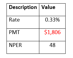

NOTE: In the above example, the pmt parameter is negative (represented by red) as we are investing the amount.

To determine the future value for the given rate, pmt and nper follow the below given steps:

Step 1: Add helper row at the bottom of table

Put your cursor below the table and add your helper row i.e., "Future Value". In this row we will type the FV formula and will fetch the future value for the given data.

Refer to the below image: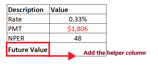

Step 2: Enter the FV formula

Move to next cell of your helper row and start typing the formula = FV(

It will look similar to the below image: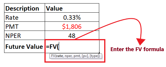

STEP 3: Add the parameter to your formula

In the first parameter, we will specify the interest rate per period. In the above table, the rate is mentioned in cell C4. So our formula becomes: =FV (C3,
Next, this function will ask for the NPER parameter. This parameter represents the total number of payment periods for the length of an annuity. The NPER is mentioned in cell C5. So our formula becomes: =FV (C3, C5
The pmt function represents the payment. Since we it an outflow so pmt is negative and is mentioned in cell C5. So our formula becomes: =FV (C3, C5, C4
Pv is an optional parameter that represents the current value, or total value of all payments. It is mentioned in cell C6. So our formula becomes: =FV (C3, C5, C4, C6)
This last parameter, i.e., type, is optional. So it will automatically take the default value 0 since we have omitted.

The overall formula will look similar to the below image: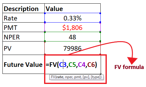

STEP 4: FV will return the output

Press the enter button as soon as you are done typing the formula. Excel will return the output for your PV formula. As shown below it will return 0 as an output of your periodic payment.

FV is $0, it implies that we will be able to repay the loan of $80,000 we had initially taken by paying 48 monthly installments of $1,806 each.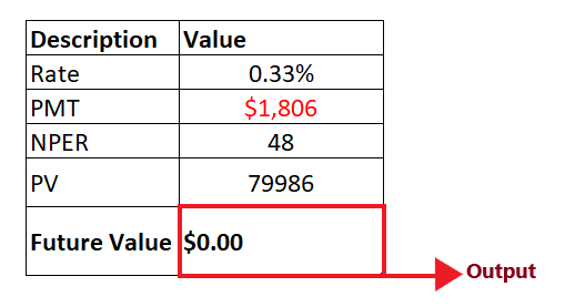

Example 2: Using the FV formula build a common calculator that calculates the future value and work well for both periodic and lump-sum investments.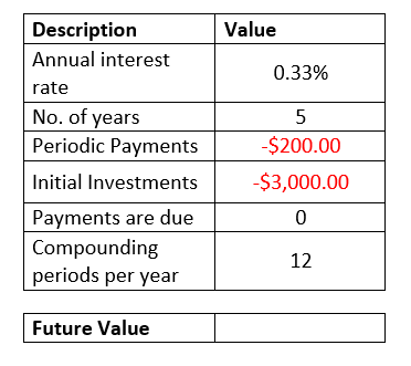

NOTE: In the above example, the pmt (periodic payments) and nper (initial investments) parameters are negative (represented by red) as we are investing the amount.

For setting up a future value calculator in Excel below the given steps:

Step 1: Add helper row at the bottom of table

Put your cursor below the table and type the heading of your helper row i.e., "Future Value". In this row we will type the FV formula and will fetch the future value for both periodic and lump-sum payments with either annuity type.

Refer to the below image: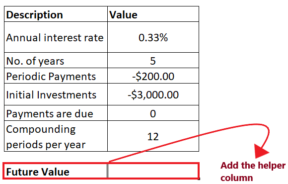

Step 2: Enter the FV formula

Move to next cell of your helper row and start typing the formula = FV(

It will look similar to the below image: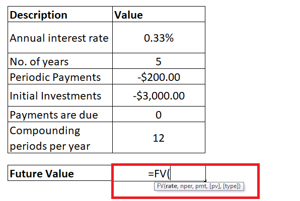

STEP 3: Add the parameter to your formula

In the first parameter, we will specify the interest rate per period. In the above table, we are given an annual interest rate. To convert the specified annual interest rate to a periodic rate, we will divide the annual rate by 12 (total periods in a year). So our formula becomes =FV (C3/C8,

NOTE: Always remember to convert annual interest rate to periodic interest rate while working with Excel FV formula for monthly cash flows.

Next, we will specify the nper To fetch the total number of periods, we will multiply the annuity term in years by 12 (total periods in a year. (nper= number of years * number of periods in a year). So our formula becomes: =FV(C3/C8, C4*C8,
Next, we will specify the pmt The negative pmt signifies an outflow payment made for each period. The pmt is mentioned in cell C5. So our formula becomes: =FV(C3/C8, C4*C8, C5,
Since the PV represents the present investment value. In our case, which is -$3000. So our formula becomes: =FV(C3/12, C4*12, C5,C6)
This annuity type is 1. The type is mentioned in cell C6. So our formula becomes: =FV(C3/12, C4*12, C5,C6,C8)

The overall formula will look similar to the below image: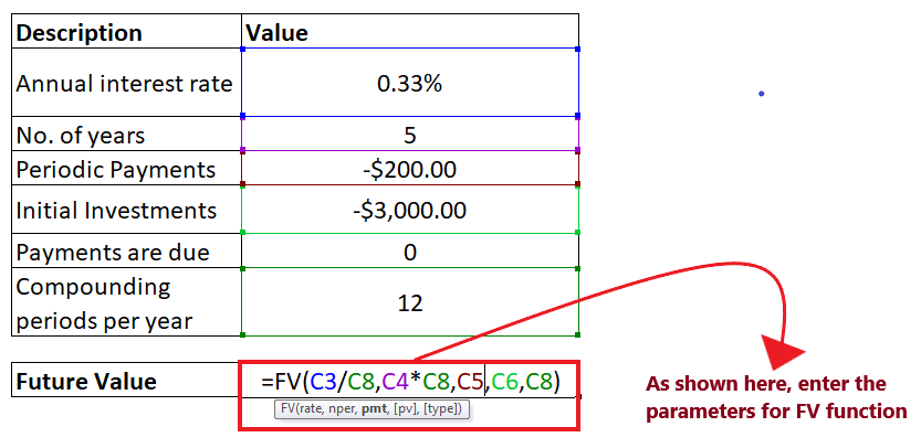

STEP 4: FV will return the output

Press the enter button as soon as you are done typing the formula. The FV calculator will return the Future value for the given data. As shown below it will return $15,151.10 as an output of your periodic payment.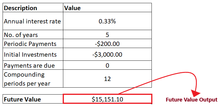

Therefore, we can conclude that the Future Value will be 15,151.10 at the end of 12 years.

Tips

In the above example, we calculated the yearly annuity. Similarly, you can find the present value for a weekly, quarterly, or semiannual annuity. To achieve this, you only need to change the number of periods per year in the respective cells.
Also, you can change the payment due to 1 if you want the cash flow to occur at the beginning of the period. You can also omit this value because it is an optional parameter and its default value is 0.

Example 3: In the below table, few of the arguments are non-numeric. Let's see what happens if you specify non-numeric arguments in NPER formula.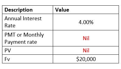

To fetch the FV output for the above table follow the below given steps:

Step 1: Add helper row at the bottom of table

Put your cursor below the table and add your helper row. In this row we will type the NPER formula and will fetch the periodic payment for the given data.

Refer to the below image: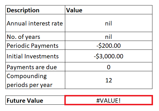

STEP 2: Add the FV formula and insert its parameters

Move the cursor of the helper cell and start typing the formula = FV(
Add all the five NPER parameters and you will receive the below formula = =FV(C3/12, C4*12, C5,C6,C8)

NOTE: We have omitted the type parameter as we have assumed the payments are due at the end of the period.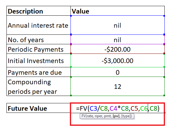

STEP 3: FV function will return #VALUE! error as Output

Press the enter button as soon as you are done typing the formula. Excel will return the output for your FV formula. As shown below it will throw the #VALUE! error.

Refer to the below image: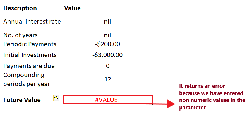

This error occurs if any of the arguments specified in your FV formula is non-numeric. To fix this error in Excel, always ensure that all the parameters are numeric and all the specified numbers are not formatted as text.

Excel FV function not working

Sometimes while working with the FV function, there are possibilities you might run into an error or a wrong result, and it mostly occurs because of one of the following reasons:

#VALUE! error

The output of FV function is a negative number or much lower than expected

This problem occurs in the FV formula when you have used positive numbers to represent the outflow payments. For example, when you calculate the payment periods for a loan, provide the pv (loan value) parameter as a positive number and the pmt argument as a negative number.

Next TopicExcel NPV Function

← prev next →