Fibonacci Retracement calculator in Excel
This tutorial covers the creation of an Excel Fibonacci Calculator. The sequence of Fibonacci numbers has many mathematical applications. The Fibonacci sequence has also been utilized in computer algorithms for calculating the golden ratio. A common analytical tool in trading is the Fibonacci Retracement. Fibonacci sequence calculations and Fibonacci calculator creation are made easy with Excel. Let's move ahead with this tutorial and learn what is meant by Fibonacci Number without any delay.
Why Is the Fibonacci Number?
The Fibonacci sequence starts with 0 and 1 as its first two numbers. The addition of the two numbers preceding it yields the next number within the sequence. The first and second Fibonacci numbers are, therefore, 0 and 1. Consequently, 0+1=1 is the following number. In the same way, 1+1=2 will be the following number. We can quickly calculate the subsequent numbers by adding the two preceding numbers.
Step-by-Step Instructions for Creating an Excel Fibonacci Calculator
Next, we'll use Excel to develop a Fibonacci calculator. We will determine retracements and extensions by utilizing the input value that indicates the upward or downward trend. To see how it functions, let's go through the steps below.
Step 1: Set the format for Fibonacci calculator
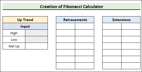
- We shall first insert the calculator's format.
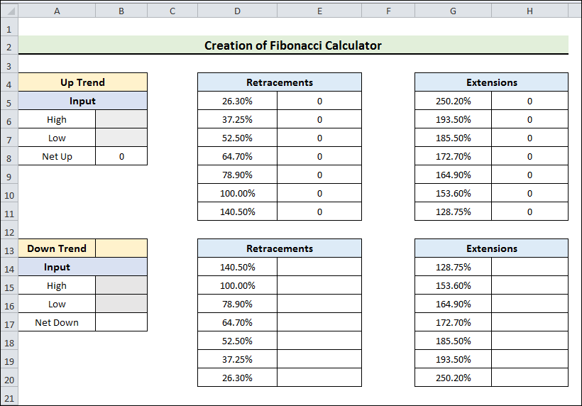
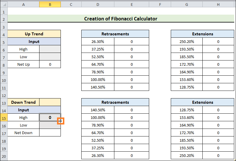
- Our format about Up Trend is shown in the following graphic.

Step2: Add Extensions and Retracements ito the Calculator
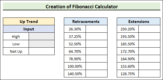
- Extensions and Retracements must be included in the calculator's format in the next step.
- The typical Fibonacci ratios in this case were 26.30%, 37.25%, 52.50%, 64.70%, 78.90%, 100%, & 140.50 %.
- Retracements will, therefore, be added appropriately.
- Next, we'll update the calculator with Extensions.

Step 3: Connect cells to create the calculator
- The input and output of the calculator will be connected in the ensuing figure.
- It would help if you established a connection between the input, retracement, and extension cells.
- In this case, our input is High and Low.
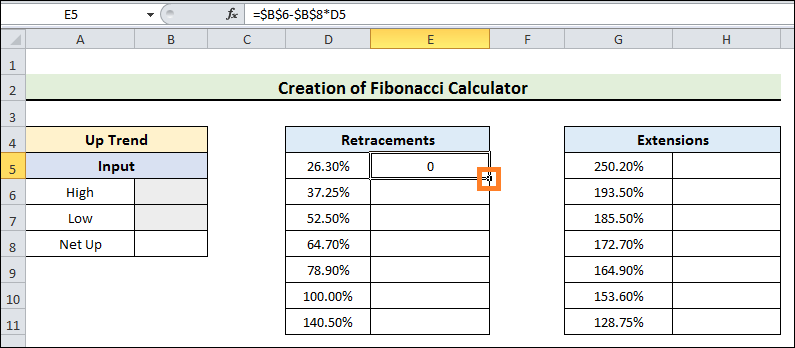
- The formula should then be entered into the E5 cell:
- To quit the editing mode, after that, hit Enter.
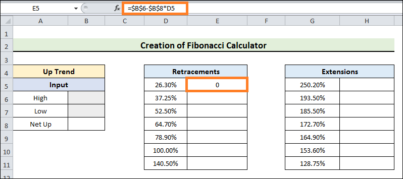
In this case, we shall apply the High Value - Net Up*Retracement formula for a particular Retracement, as indicated by $B$6-$B$8*D5.
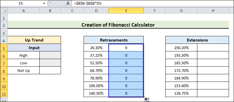
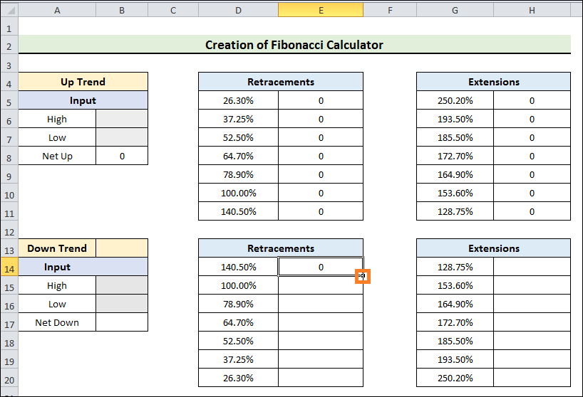
- The following (+) icon will then drag down the formula within the Retracements column.

- So, the column receives an application of the formula.
- Since the input value hasn't been added yet, the column displays 0.

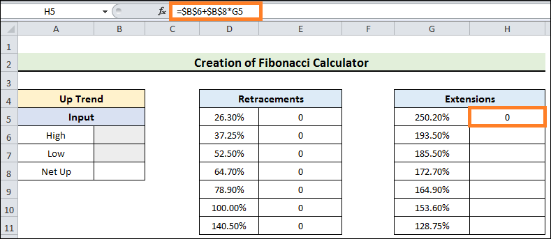
- Write the formula within the H5 cell in the subsequent step.
- To quit the editing mode, after that, hit Enter.

This time, the formula for a certain Extension-High value + Net Up*Extension-will be applied, as indicated by $B$6+$B$8*G5.
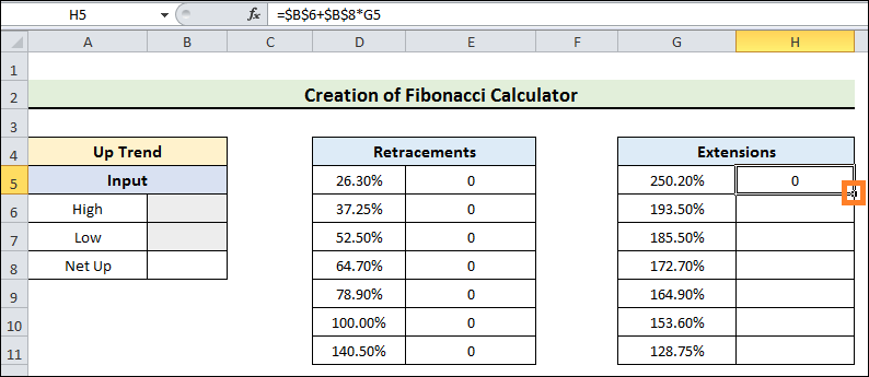
- Utilize the Fill Handle to drag the formula down into the Extensions column.

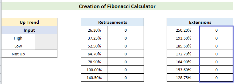
- The formula is then added for the Extensions column as a consequence.
- However, because we forgot to enter the number in the input, the result is 0 instead of 1.

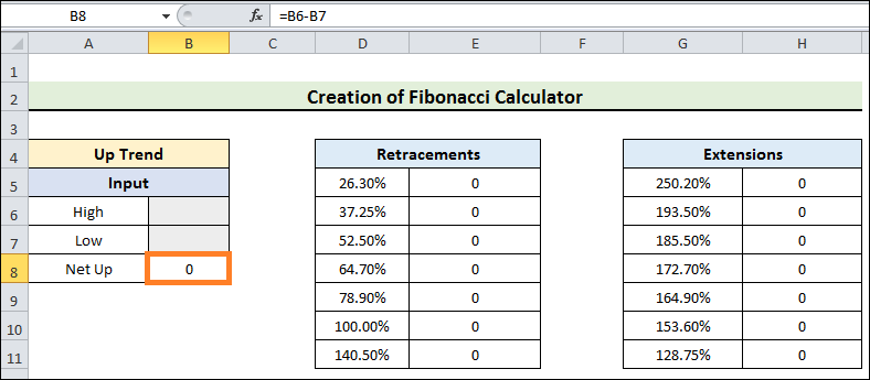
- Net Up's value is required in the following step.
- This means that we must figure out what Net Up is worth.
- Put this formula within the B8 cell, then:
- Click Enter after that to continue.

Step 4: Set Up the Format for the Down Trend
- Similarly, we will include Retracements and Extensions for the Down Trend.

- The algorithm for calculating Retracements of the Down Trend must be written down in the next step.
- Consequently, enter the subsequent formula in the field E14:
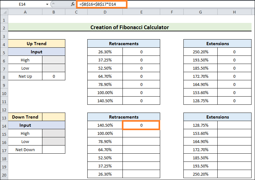
Thus, $B$16+$B$17*D14 As shown by E14, we are applying the formula Low Value + Net Down*Retracement for a particular Down Trend's Retracement.
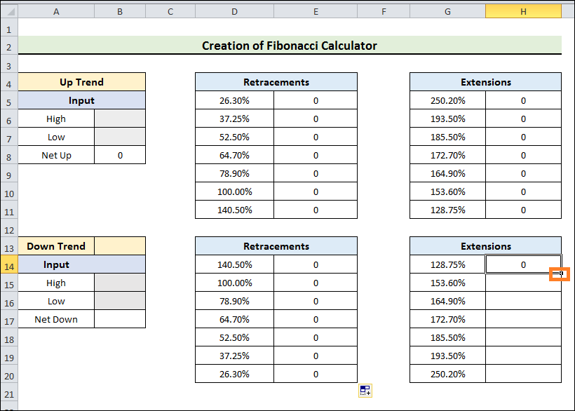
- Next, drag the formula down in the Retracements column using the Fill Handle.

- We now have to put the formula for figuring out Extensions of the Down Trend in writing.
- Consequently, enter the subsequent formula into the H14 cell:
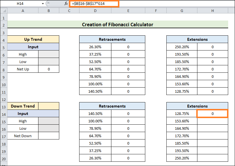
Here, $B$16-$B$17*G14 denotes that we are applying the Low Value - Net Down*Extension calculation for a particular Down Trend's Extension.
- Next, use the Fill Handle to move the formula down in the Extensions column.

- However, we do not wish to insert an input twice.
- We want to display the output for the retracements and extensions of up and down trends and insert the input just once.
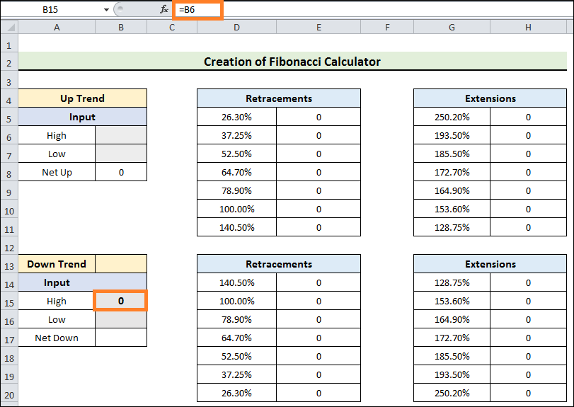
- Link each input of the Up Trend & Down Trend as a result.
- Thus, enter the following formula within the formula bar of the C15 cell:
- To end the editing mode, hit Enter after that.
- Consequently, the input we insert into the B6 cell will be displayed within the B15 cell.

- Next, connect the Low and Net numbers by dragging down the formula with the Fill Handle.

Final Result
- The Fibonacci Calculator is now complete.
- The input must now be inserted into cells B6 and B7.
- Therefore, the outcome will be displayed by placing the High value into B6 & the Low value in B7.
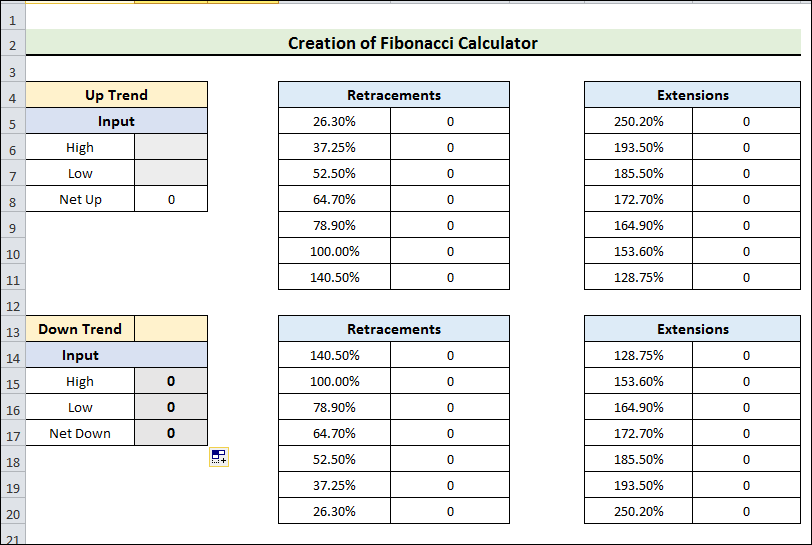
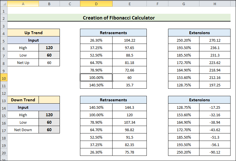
- Enter 120 as the High value and 60 as the Low value to check the calculator.
- As a result, both down and up trend extensions and retracements are visible.

- Look for a different value once again.
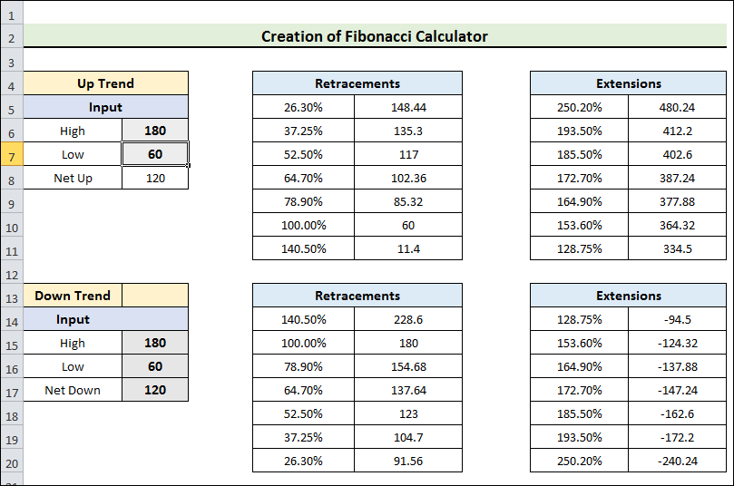
- Insert, therefore, 180 for the High value and 60 for the Low value.
- As a result, both down and up trend extensions and retracements are visible.

How to Use Excel to Create the Fibonacci Sequence
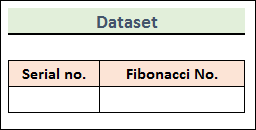
Let's create the Fibonacci Sequence using Excel. The serial number will appear in the first column, and the matching Fibonacci number will appear in the second. Let's see how it functions by going through the stages below.
Step 1: Enter the Initial Sequence of Fibonacci Number
- First, the first two numbers in the Fibonacci sequence must be entered.
- The Fibonacci sequence's first two numbers are 0 and 1.
- Thus, enter the value 0 in cell B5.
- This suggests that the first number of the Fibonacci sequence is 0.
- Likewise, enter 1 as the input in the B6 cell.
- The statement suggests that the second number of the Fibonacci sequence is 1.
- We're going to present the subsequent Fibonacci series components to you now.

Step 2: Use the formula to get the next sequence
- The sequence's third number will be determined in the phase that follows.
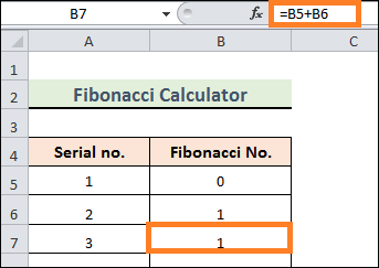
- In the B7 cell's formula bar, enter the following formula.
- Consequently, the Fibonacci sequence's third serial is visible.

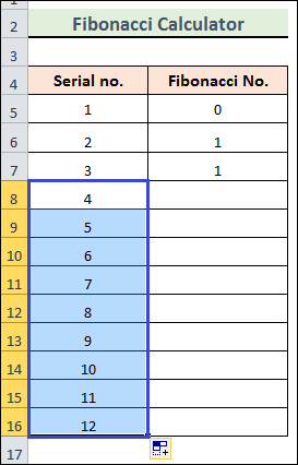
- We may create the Serial column using Excel and enter the serial number automatically rather than by hand.
- To progressively expand the Serial column, enter the subsequent formula into the A8 cell:
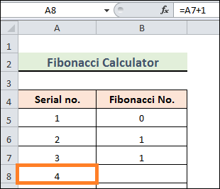
- The serial number will be generated in the next step by dragging down the formula into the Serial column with the help of the (+) icon.

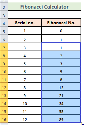
- Similarly, we will drag down the Fibonacci number sequence formula in the Fibonacci Number field.

Output
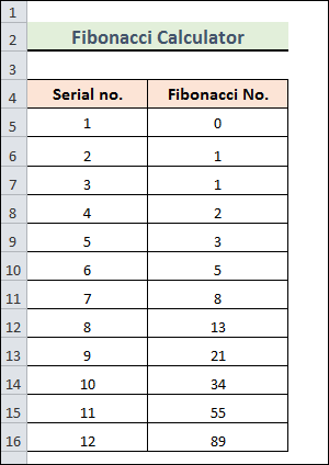
- With Excel, we can now finally determine the Fibonacci number.
- The sequence can be extended to meet your needs by using the drag-down option.

|


 For Videos Join Our Youtube Channel: Join Now


