| |

UNIQUE function: a quick method to find a unique value in Microsoft ExcelIn this respective tutorial, we will be looking at how we will be getting a unique value in Microsoft Excel by making use of the UNIQUE function as well as the dynamic arrays effectively; we will be learning a simple formula to find unique values in a column or row, in the multiple columns, which are based on conditions, and a lot more as well. Moreover, it was known that, in the previous versions of Microsoft Excel, extracting a list of unique values was also a hard challenge. In this, we will see how one can easily discover the uniqueness that occurs just once, extracting all the distinct items in a list, ignoring the blanks, and much more. Every task required combining several functions and a multi-line array formula that only Excel gurus can fully understand. Besides, introducing the UNIQUE function in Microsoft Excel 365 has changed everything! What used to be rocket science becomes as easy as ABC, respectively? Now, we don't need to be a formula expert to get a unique value from a range based on one or multiple criteria and arrange the results alphabetically.
What do you mean by UNIQUE Function in Microsoft Excel?It was well known that the respective UNIQUE function in Microsoft Excel returns a list of the unique values from a given range or array, as it works with any data which are as follows:
And the function is primarily categorized under the Dynamic Arrays of Function as well as the result is a dynamic array that automatically spills into the neighboring cells vertically or horizontally, respectively. Syntax: The syntax that can be used for the UNIQUE function in Microsoft Excel is as follows: In which,
Important Note. The respective UNIQUE function is only available in Microsoft Excel for Microsoft 365 and Excel 2021 versions. And the Microsoft Excel 2019 and 2016 version and earlier does not support dynamic array formulas, so the UNIQUE function is not available in these versions effectively. What are the Basic UNIQUE formulas that are used in Microsoft Excel? Below is an Excel unique values formula in its simplest form respectively. And the main goal is to extract a list of unique names from the given range from B2:B10. For this, we need to enter the following Formula in the column D2: =UNIQUE (B2:B10) And it should be noted that the 2nd and the 3rd arguments are omitted because the defaults work perfectly in our case as well: as we are comparing the rows against each other and wish to return all the different names in the range respectively. After that, when we press the Enter button from our keyboard to complete the Formula, Excel will output the first found name in D2 spilling the other names into the cells mentioned below. As a result, we have all the unique values in a selected column as well: 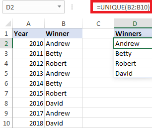
If in case our data is across the columns from B2 to I2, set the 2nd argument to TRUE to compare the columns against each other: =UNIQUE (B2:I2, TRUE) And then, we will type the above Formula in cell B4 and press Enter, and the results will spill horizontally into the cells to the right position as well. Thus, we will get the unique values in a row respectively: 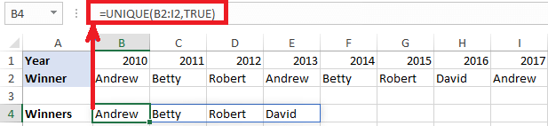
UNIQUE FUNCTION: Important notes and tipsIn Microsoft Excel, the UNIQUE function is considered the new function, and just like other dynamic array functions, it also has a few specificities that we all should be aware of:
How can one find unique values: formula examples?The examples below will show some more practical uses of the UNIQUE function in Microsoft Excel. And the main idea is to extract the unique values or remove the duplicates as well, depending upon our own viewpoint, in the simplest possible way. How can one extract unique values that occur only once? To get a list of values that will be appearing in the specified range exactly once, will set the 3rd argument of UNIQUE to TRUE. For example: To pull the names which are on the winners list one time, we will be making use of this Formula respectively: In which the cell ranging from B2:B10 is the source range and the 2nd argument (by_col) is FALSE or omitted because our data is organized in rows. 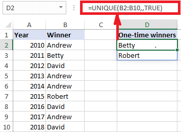
How can we find the distinct values that occur more than once in the Excel sheet? If in case we are pursuing an opposite goal, that means we are looking to get a list of values that will be appearing in a given range more than one time, then we will be making use of the UNIQUE function together with FILTER as well as with the COUNTIF function:
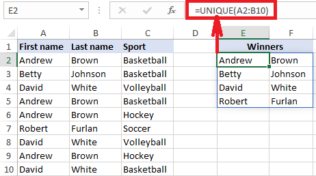
Working of the above Formula It was well known that, at the heart of the Formula, the FILTER FUNCTION filters out all the duplicate entries, which are based on the count of occurrences and are returned by the function: COUNTIF FUNCTION. As in our case, the outcome of the COUNTIF is this array of counts as well: {4;1;3;4;4;1;3;4;3} And the comparison operation (>1) changes the above array to TRUE and also to the FALSE values, in which the TRUE represents the items that appear more than once: {TRUE;FALSE;TRUE;TRUE;TRUE;FALSE;TRUE;TRUE;TRUE} This particular array is handed off to the FILTER as the include argument, telling the function which respective values to include in the resulting array as well: {"Andrew";"David";"Andrew";"Andrew";"David";"Andrew";"David"} And we can notice that only the values corresponding to TRUE will survive effectively. Moreover, the above array moves to the array argument of the UNIQUE function, and after removing duplicates, it outputs the final result efficiently: {"Andrew";"David"} Note: It should be noted that, similarly, we can easily filter out the unique values which will occur more than twice or more than three times, etc. For this, we can change the number in the logical comparison respectively.How can we find the unique values in multiple columns (unique rows) in Microsoft Excel? In this particular scenario, when we want to compare two or more columns and returning out the unique values between them, then in that scenario, we can easily include all the target columns in the array argument as well. And for instance, if in case we want to return the unique First name (column A) and the Last name (column B) of the winners, then in that case, we will be entering this Formula in the cell that is E2: =UNIQUE (A2:B10) After that, we will press the Enter key from the keyboard to yield the following outcome as well: 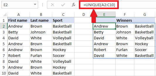
And to get the unique rows, which means that the entries with the unique combination of values in columns A, B, and C, these are the formulas that need to be used: =UNIQUE (A2:C10) 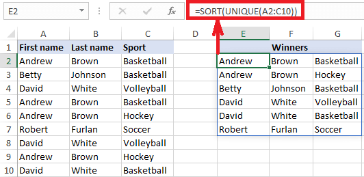
How can one easily get a list of unique values sorted alphabetically in Excel? How do we usually alphabetize in Microsoft Excel? It is like, just by using the inbuilt features in Excel that is none other than the: Sort or the Filter. And the problem that is associated with this is that we need to re-sort every time our selected source data changes because, unlike Excel formulas that recalculate automatically with every change in the worksheet, the features have to be re-applied manually efficiently. Moreover, with the introduction of the Dynamic array function, the above problem can be easily sorted. But what we need to do is simply just wrapping out the SORT function around a regular UNIQUE formula, as like this: SORT (UNIQUE (array))
=SORT (UNIQUE (A2:C10)) Compared to the above example, the output is much easier to perceive and work with. For instance, we can see that Andrew and David have been winners in two different sports as well: 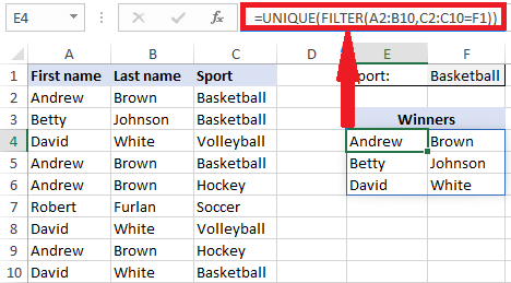
Important Tip. In this example, we have usually sorted the values in the 1st column from A to Z, which are the defaults of the SORT function; therefore, the optional sort_index and sort_order arguments are omitted. How to find out the unique values in multiple columns and concatenate them into one cell? While searching in multiple columns, the Microsoft Excel UNIQUE function outputs each value in a separate cell by default. Perhaps, we will find it more convenient to have the results in a single cell And to achieve this, instead of referencing the entire range, we can use the ampersand (&) to concatenate the columns and put out the desired delimiter in between, respectively. As an example, we concatenate the first names in the cell ranging from A2:A10 and the last names in the cell ranging from B2:B10 and then separate the values with a space character (" "): =UNIQUE (A2:A10&" "&B2:B10) And as an outcome, we can have a list of full names in one column effectively: 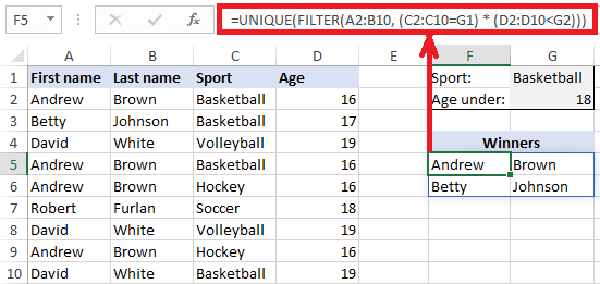
How can we get a list of the unique values based on the various criteria? To extract the unique values with a condition, we can make use of the Excel UNIQUE as well as the FILTER functions both together:
Here is the generic version of the filtered unique values formula respectively: UNIQUE (FILTER (array, criteria_range = criteria))
=UNIQUE (FILTER (A2:B10, C2:C10=F1)) A2:B10 is a range that can be used to find the unique values, and C2:C10 is the range to check for the criteria. 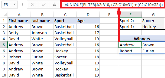
How can one filter unique values which are based on multiple criteria? And to find out the unique filter values with two or more conditions, we can make use of the expressions shown below to construct the required criteria for the FILTER function respectively: UNIQUE (FILTER (array, (criteria_range1 = criteria1) * (criteria_range2 = criteria2))) And the result of the Formula is a list of unique entries for which all specified conditions are TRUE. In terms of Microsoft Excel, this is also called the AND logic. And to see the Formula in action, let us get a list of unique winners for the sport in G1 (criteria 1) and under age in G2 (criteria 2): With the source of the range in A2:B10, sports in C2:C10 (criteria_range 1) and ages in D2:D10 (criteria_range 2), and the formula takes this form: =UNIQUE (FILTER (A2:B10, (C2:C10=G1) * (D2:D10<G2))) And it returns exactly the results we are looking for: 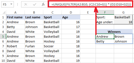
Working of the above Formula Here is a high-level explanation of the Formula's logic: So in the respective include the argument of the FILTER function, we will be supplying out the two or more range/criteria pairs. And the result of each logical expression is an array of TRUE and FALSE values. The multiplication of the arrays coerces the logical values to numbers and produces an array of 1s and 0s. Since multiplying by zero always gives the zero, only the entries that meet all the conditions have 1 in the final array. The FILTER function will then filters out the items corresponding to 0 and hand off the results to UNIQUE respectively: How to find out the Filter unique values with multiple OR criteria? And to get a list of unique values which are based on the multiple OR criteria, i.e., when this OR that criterion is TRUE, we will be adding the logical expressions instead of multiplying them as well: UNIQUE (FILTER (array, (criteria_range1 = criteria1) + (criteria_range2 = criteria2)))
=UNIQUE (FILTER (A2:B10, (C2:C10="Soccer") + (C2:C10="Hockey"))) If needed, we can, of course, enter the criteria in separate cells and refer to those cells shown below respectively: =UNIQUE (FILTER (A2:B10, (C2:C10=G1) + (C2:C10=G2))) Working off the above Formula: It is just like when we are testing out the multiple AND criteria, and we can easily place out the several logical expressions in the include the argument of the FILTER function, each of which returns an array of TRUE and FALSE values. When these arrays are added up, the items for which one or more criteria are TRUE will have a value of 1. The items for which all the criteria are FALSE will have the value 0. As the outcome, any entry that meets any single condition makes it into the array handed over to the UNIQUE function efficiently. How can we get unique values in Microsoft Excel, ignoring blanks? If we are working with a set of data that primarily contains some gaps, a list of unique obtained with a regular formula is likely to have an empty cell or zero value. And this happens because the Microsoft Excel UNIQUE function is designed to return all distinct values in a range, including blanks. So, if our source range has zeros and blank cells, the particular unique list will contain 2 zeros, one representing a blank cell and the other: a zero value. And additionally, if the source data is containing out the empty strings returned by some formula, the unique list will also include an empty string ("") that visually looks like a blank cell as well: 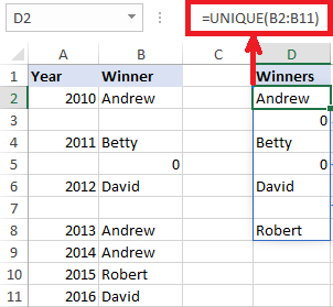
And to get a list of unique values without blanks, then, in that case, we need to do the following things as well:
And in a generic form, the Formula will look like as: UNIQUE (FILTER (range, range<>")) Moreover, in this example, the Formula in the cell D2 is: =UNIQUE (FILTER (B2:B12, B2:B12<>"")) And as the outcome, Excel returns a list of unique names without empty cells: 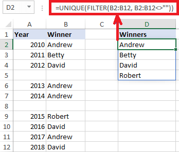
How can one find the unique values in specific columns in Excel? Sometimes, we may want to extract unique values from two or more columns that are primarily not adjacent. We may also want to re-order the columns in the resulting list at that time. Both tasks can be fulfilled with the help of CHOOSE function. UNIQUE (CHOOSE ({1, 2,},range1, range2)) And from our sample table, let us suppose we wish to get a list of winners that are based on the values in columns A as well on C and arrange out the results in this order: first a sport (column C), and then a sportsman name (column A). To have it done, we construct this Formula as follows: =UNIQUE (CHOOSE ({1, 2}, C2:C10, A2:A10)) And will get the following result: 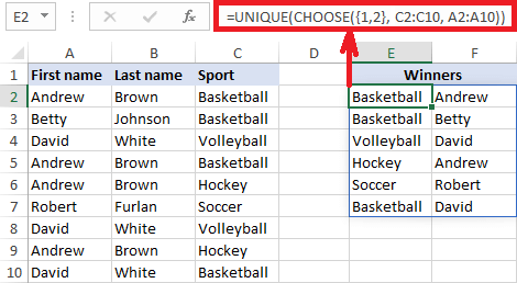
|
 For Videos Join Our Youtube Channel: Join Now
Feedback
- Send your Feedback to [email protected]
Help Others, Please Share


