How to implement Left LOOKUP in Excel

VLOOKUP is one of the most commonly used Excel functions that looks up data in a table organized vertically (or towards the right). What if, instead of right, we want to look up a value in your table and return its corresponding value to the left? To counter this problem, Excel has not provided any predefined formula until Excel 365 or Excel 2021. In earlier versions, Left Lookup can be achieved simply by combining the INDEX and MATCH functions.

But now you no longer need to combine those two functions as only one function will cater those requirements. All you need to do is to specify the lookup table, and XLOOKUP will handle the remaining task for you.

In this tutorial, we will learn the step-by-step implementation of both the methods to get the Left LOOKUP function.

1. Left Lookup using Index and Match functions
2. Left lookup performed natively with XLOOKUP function

Left Lookup using Index and Match functions

For the previous Excel versions (until Excel 365 and Excel 2021), Microsoft has not introduced any particular formula that could handle the left lookup operations. If you are working with previous Excel working, you can incorporate left lookup by combining INDEX and MATCH functions.

But before stepping ahead, let's cover what INDEX and MATCH functions are:

What Is INDEX function?

"The INDEX function in Excel is an inbuilt function that returns the value at a specified location in a given array or range of cell. This function is also used to retrieve individual values, or entire rows and columns."

Syntax

Parameter

1. Array (required) - This parameter represents a range of cells, or an array constant.
2. row_num (required) - This parameter represents the row position in the given array.
3. col_num [optional] - This parameter represents the column position in the specified array or range of cells.

Returns

This function returns the value of a lookup data in the specified table or an array, selected by the row and column number indexes.

What is MATCH function?

The Excel MATCH function is used to determine the position of an item in a range. It returns the position of a value found in the specified lookup_array. For example, we can use MATCH to find the position of the item "mobile phone" in this list of electronic items.

Syntax

Parameter

1. lookup_value (required) - This parameter represents the value that the user wants to match in lookup_array.
2. lookup_array (requird) - This parameter represents a range of cells or an array reference.
3. match_type [optional] - This parameter can accept four values depending upon your requirement; if you skip this argument, by default, it takes 0 as its value and returns an exact match.
   • 0 - You can enter this value if you want an exact match.
   • -1 - You can enter this value if you are looking for an exact match or next smaller. It returns the next smaller value, if it not founds and exact match.
   • 1 - You can enter this value if you want to return an exact match or next larger value. If an exact match is not found, the next larger value is returned.
   • 2 - This value represents the wildcard character match.

Returns

The Microsoft Excel Match function returns a number representing that position of an item found in lookup_array.

Steps to implement LEFT LOOKUP Function

Since we have already covered the basic information about the INDEX and MATCH functions, let's combine them in a single formula.

Consider the following data, a table showing the list of equipment utilized in hospital industries and their current status, like whether the products are available, or are in transit, or none.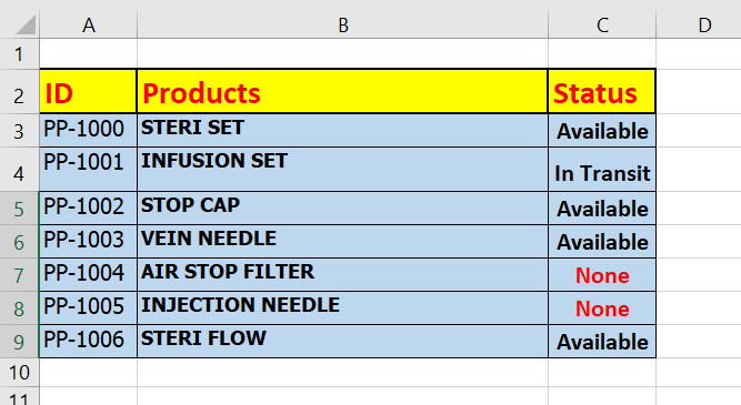

What is we want to quickly check the status of some of the equipment through their product_ID? We can do the same using the left Lookup.

Perform the following steps:

STEP 1: Incorporate the MATCH function

The first step is to incorporate the Excel MATCH function. We will use the below formula wherein we will specify the row number and Array to match the value.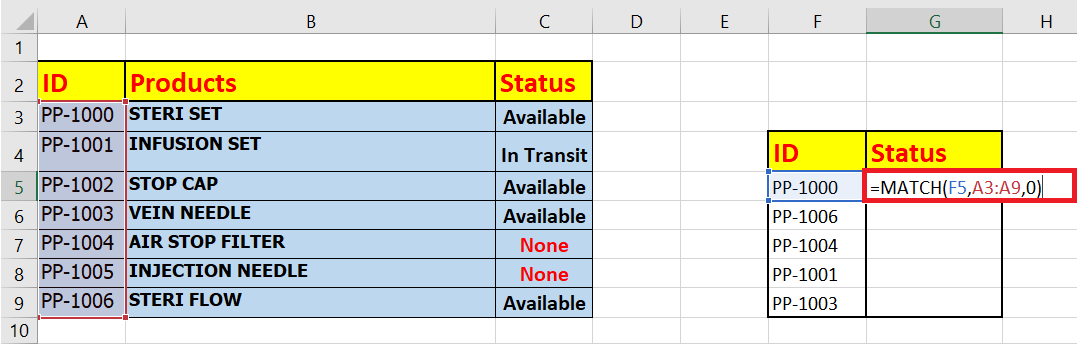

As a result, it will return the position of the value that you want to match in the given array. In our case it has returned 1, it means the value 101 is found at position 1 in the specified range A3:A9.

STEP 2: Merge MATCH with INDEX function

Next, we will combine the output of Match function with the INDEX function. In terms of Index function, we will use the specify the array and row number.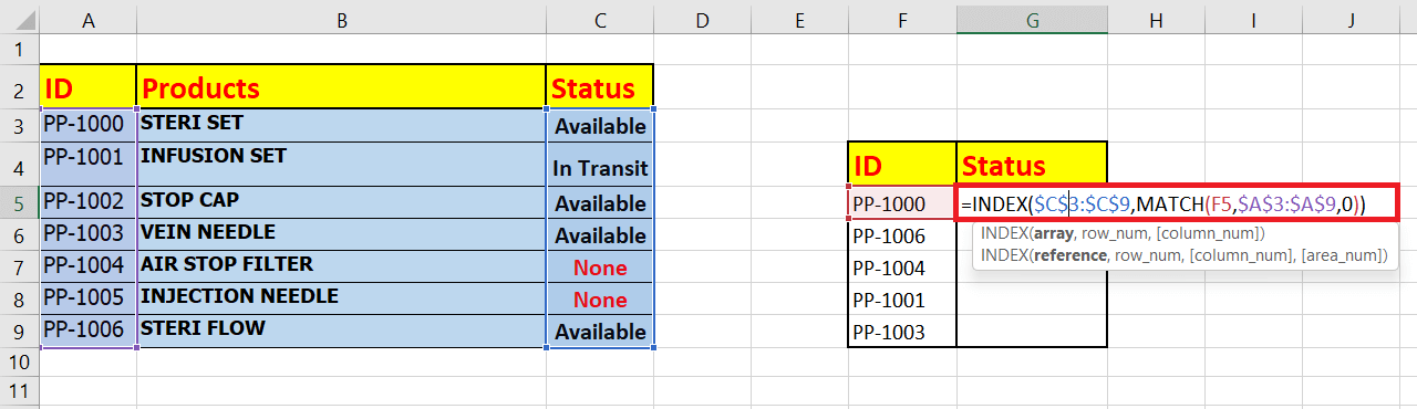

Step 3: Returns the status value

As a result, the above formula will quickly look for the first element in the specified array (C3:C9), and will return the status. In our case, we will get the following result.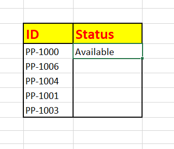

Step 4: Drag the formula in cell B2 down to cell B11.

Next, to replicate the formula down the cells, we will drag the above formula down. Since we have used absolute references for the lookup_array range (($C$3:$C$9, $A$3:$A$9 ) therefore, it won't change and remains the same, while the relative reference (F5) changes as you drag down.

It will return the following output: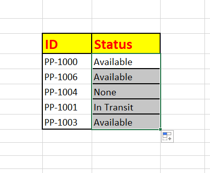

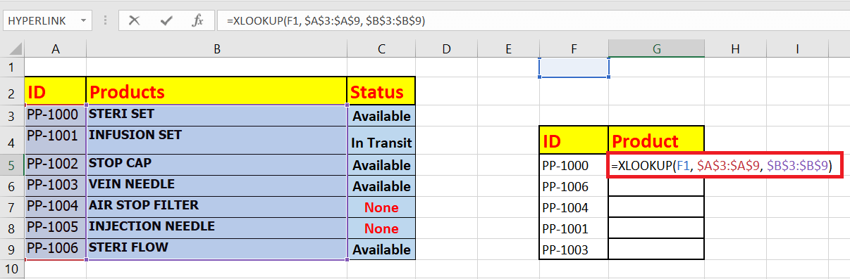
To summarize the above formula, the match function matches the values with the given array_range and returns its position. The INDEX functions to get a value at a given location in a range of cells based on numeric position.

XLOOKUP to perform a Left Lookup

If you have Excel 365 or Excel 2021, simply use the XLOOKUP function to perform a left lookup.

"The XLOOKUP function in Excel looks at a range or an array for a given value and returns the corresponding value from another column."

The advantage of using this function is that it can look up both the positions in your table, i.e., vertically and horizontally, and can perform either an exact match (default), an approximate match (the closest data is found), or a wildcard match (using wildcard characters a partial match is found).

Syntax

Parameters

1. Lookup_value (required) - This parameter represents the value to search for in the table.
2. Lookup_array (required) - This parameter represents the table or the range or array where to search.
3. Return_array (required) - It signifies the range or array from where the values will be returned.
4. If_not_found [optional] - This is an optional parameter that represent a value that will be returned if the match is not found. In case you have skipped the parameter, the #N/A error is returned.
5. Match_mode [optional] - This parameter can accept four values depending upon your requirement; if you skip this argument, by default, it takes 0 as its value and returns an exact match.
   • 0 - You can enter this value if you want an exact match.
   • -1 - You can enter this value if you are looking for an exact match or next smaller. It returns the next smaller value, if it not founds and exact match.
   • 1 - You can enter this value if you want to return an exact match or next larger value. If an exact match is not found, the next larger value is returned.
   • 2 - This value represents the wildcard character match.
6. Search_mode [optional] - This parameter helps the user to manage the direction of search. if you skip this argument, by default, it takes 1 as its value and starts the search from first to last position of your array. It can take the following values:
   • 1 - Putting this value will start the search from first to last position of the defined array.
   • -1 - Putting this value will start the search in reverse order i.e., from last to first position.
   • 2 - This value is used if you want to have a binary search where the data is sorted in the ascending order.
   • -2 - This value is used if you want to have a binary search where the data is sorted in the descending order.

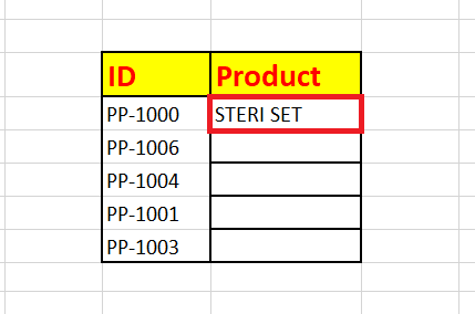
Returns

The XLOOKUP function searches a range or an array for predefined value and it returns the related value from another column.

Example

For example, let's add the products column to the left of our sample table. We aim to get the product name based on the id number.

The Xlookup formula will be as follows:

Below are the steps:

1. Enter the formula in your Excel cell and press the enter button.
   
2. As a result, it will return the Products name for the given id.
   
3. Drag the formula the above formula down. Since we have used absolute references for the lookup_array range therefore, it remains the same, while the relative value changes.

Just a single formula, and you are done! So if you are using previous Excel versions, quickly upgrade to newer versions; also, Microsoft has introduced various other functions and features with the latest versions. But until then, go ahead and give Left lookup a try!