Formula Auditing in the Microsoft Excel

It is well known that why Microsoft Excel is much popular throughout the world, it is because of its wide range of formulae, functions, as well as macros. And these can handle almost every task in the world very smoothly respectively. All these available formulae are pretty easy to use, but it becomes challenging when we efficiently use multiple procedures in combination. And sometimes, it does not give out the result outcomes as expected by an individual.

Moreover, it becomes effortless and straightforward to trace back the particular amount of occurred errors if the used formulae are pretty simple. However, when we start creating complex procedures, it becomes hectic for us and any individual to track the mistakes with such recipes. And hence, it is said there it is essential for any particular user to trace all the errors respectively.

Besides all these, Microsoft Excel provides a huge variety of built-in tools which allow as well as to individual for auditing errors with the Help of the various formulae and corrected ones.

And on moving further, we primarily have six main tools under Microsoft Excel to do the formulae auditing, which as listed below:

1. Trace Precedents.
2. Trace Dependents.
3. Remove Arrows.
4. Show Formulas.
5. Error Checking ( that includes the Error Checking, Trace Error as well as the Circular References)
6. Evaluation of the formulas.

Now let us explore each formula mentioned above, auditings one after the other under the shades of Microsoft Excel.

# Examples of the Auditing tools in the Microsoft Excel

Let us now discuss the various examples of the Auditing Tools used in Microsoft Excel.

Example # 1: Trace Precedents

Trace precedents can be effectively defined as the individual cells affecting the values or the formulae present under the selected cell. Let us now we will considered that we have five Principle amounts which we can effectively invest with a rate of interest that is 12% and for six years respectively, And we have calculated the interest amounts for the entire five available principles amount using a simple formula that is:

Principle*Interest Rate*Period (in years)

As can be effectively depicted in the below figure,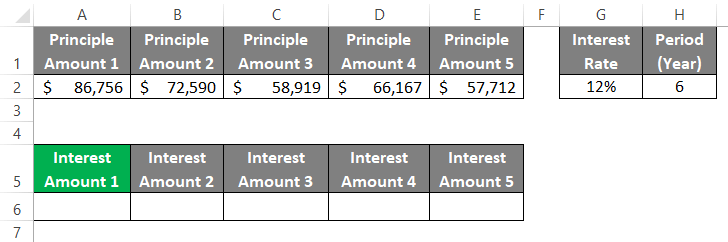

Just after that, if we click on the cell that is cell A6 and will press F2, then after pressing we can see that the formula which we can use to capture Interest Amount 1, can be efficiently seen in the below depicted screenshot.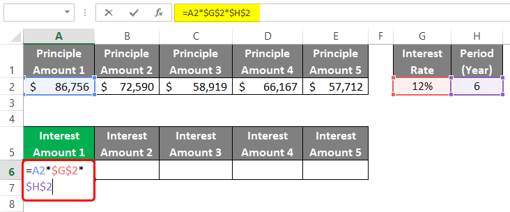

And it will depict us that the respected Interest Amount 1 is primarily based on Principle Amount 1 Value (A2) and also on the Interest Rate (H2) for the Period (I2). However, Microsoft Excel has its way of showing this relationship through the Help of the cell precedents present under the formula auditing group respectively.

Step 1: Select the cell A6 from the available worksheet and click on the Formulas tab present on the Microsoft Excel ribbon.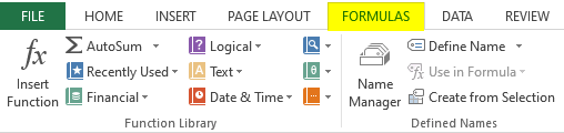

Step 2: Once we will click on the Formulas tab, we can see the Formula Auditing group, which is present just under it with the different formula auditing options which are efficiently available.

Step 3:Now, in this particular step, we will be clicking on the Trace Precedents option, that are basically present just under the Formula Auditing group, and then eventually it will make a connection between all the individual cells that are affecting the currently selected cell through blue-colored arrows as clearly depicted in the below-attached screenshot: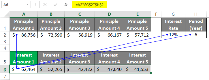

The particular Trace Precedents will help us (or an individual) find out the cells associated with the specific formula using which the values are obtained respectively.

# Example 2: Removing Arrows

It was well known that the "Trace Precedents" were excellent and sound since they allowed an individual or us the efficient relationship between the different cells present inside our Microsoft Excel sheet.

However, we don't want these things in our file as it was practically not required in any scenario, and thus we wanted to remove it. So, whether Is it Possible? Well, possible! Let us now understand this,

An individual or we must move or go again to the Formula Auditing group (In which we will select out the Formulas tab through the Help of the ribbon, and if we are not there and also we can see this group within it respectively). After that, we need to click on the "Remove Arrows dropdown," as depicted in the figure below.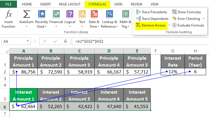

And once we click on the respective Remove Arrows dropdown, then we can see the list of options, which are seen in the below-attached screenshot effectively: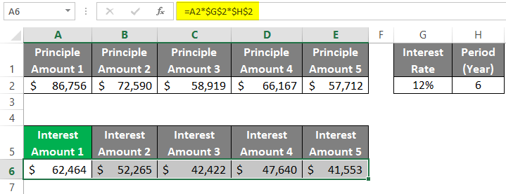

And soon, we can either hit the first option, which is capable of removing all the arrows (precedents as well as dependents one in the Microsoft Excel sheet), or else we can select the particular options that will remove the precedents or the dependents efficiently.

# Example 3: Trace Dependents in the Microsoft Excel

Now, let us suppose that we randomly click on any particular cell of the Microsoft Excel sheet, and we want to check out the cells that depend on the currently selected cell. So now the question arises: Can we do that in Microsoft Excel?

And the answer to the above particular questions is that: Yes, it is possible to do, It was well known that the particular Trace Dependents is the significant function that shows an individual or us a relationship between the specifically selected cell and all other cells with an efficient dependency on the selected cell.

Now on moving further, Let us suppose that we have selected out the cell, which is the cell H2 (Interest Rate). And we wanted to check out what are all the other cells that have a dependency on H2, and this could be easily attained or accomplished by an individual or us in Microsoft Excel by just following the below-mentioned steps which are as follows:

Step 1: First of all, we will select the cell which is none other than the cell that is cell G2 which is present in our Microsoft Excel sheet, as seen in the figure attached below.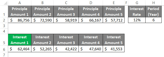

Step 2:Now, after that, we will click on the Formulas tab, which is present on the Microsoft Excel ribbon, and then from there, we will select the Trace Dependents to see what all are the cells that are primarily dependent on the cell G2, as it was depicted in the below-attached screenshot: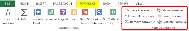

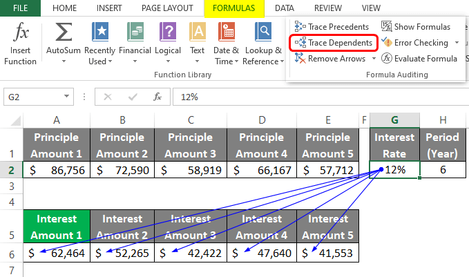
And after that, once when we click on Trace Dependents, and then we will be able see all the individual cells which have an efficient dependency on the cell that cell G2, and they will be connected with blue arrows.

# Example 4: How to Show Formula in the Microsoft Excel

Now, we will see that Formulas is an exciting feature within the respective Microsoft Excel that will show us the formulas present under all cells (formulated) instead of the values efficiently.

We need to go to the Formulas tab through the Microsoft Excel ribbon. After that we will be clicking on the Show Formulas button which is present just under the Formula Auditing group in order to see all the formulas in the current Microsoft Excel sheet respectively, as depicted clearly in the below attached figure.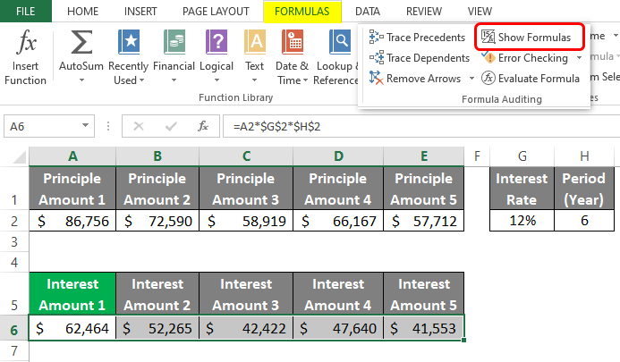

And once we click on the particular "Show Formulas button," we can see all the formulated cells with formulas instead of values, as clearly seen in the screenshot below.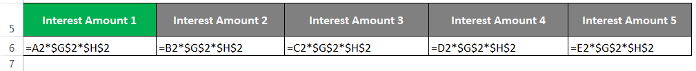

# Example 5: Error Checking in the Microsoft Excel

Let us assume that we have two respective numbers which are, Number 1 and Number 2, respectively, as seen in the screenshot below.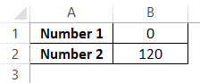

After that, we will call the function that takes these two particular cell references, and we should give some of the output. We will be using the ROUNDUP function in Microsoft Excel. As could be seen in the cell B3; for more references, it can be seen in the below-attached screenshot: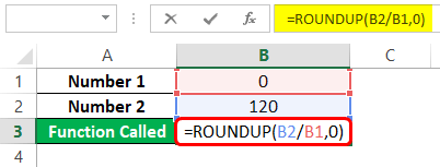

We should make use of the ROUNDUP function that can be used to divide 120 by zero and round it up to the nearest integer. And after that, we will "Hit" enter in order to see the output of this formula, as depicted in the screenshot below.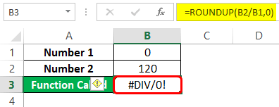

Oh, Crap! We are getting an error here too. How to check the error? Well, Excel has an Error Checking option with it.

1. Now we are moving to the Formula Auditing group, and then we will click on the Error Checking button, as seen in the screenshot below.

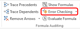
The Error Checking dialogue box will appear on the screen, as seen in the screenshot below.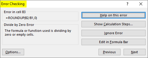

Now we can see that we can get online Help on this error by clicking on the "Help" on this Errorbutton, or else we can see the calculation steps which are involved in this error by hitting out Show Calculation Steps, or we can ignore the error or Edit the formula as well.

After that, we will click on Help on this Error button, and we will be redirected to the Office Support online page, as shown below in the attached screenshot.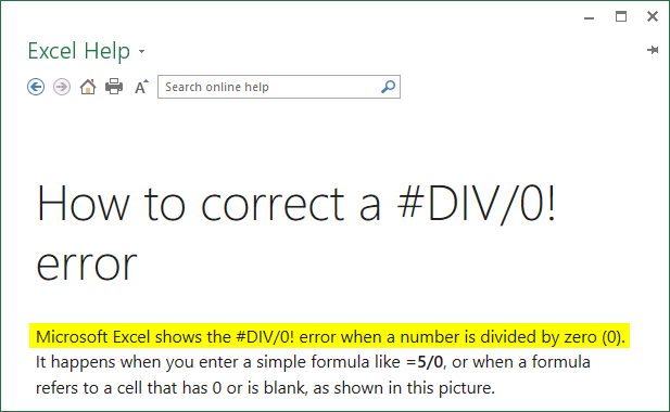

From here, we will get the #DIV/0! An error occurs when we try to divide some of the numbers with zero. And then, we will change out the value of Number 1 under cell B1 and see how the formula works in B3, as clearly depicted in the below-attached screenshot.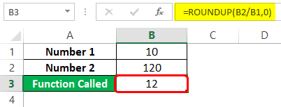

This is how error checking will help us in Microsoft Excel.

Things to Remember

The following things or the important points that must be remembered by any of the individual who is working with the Auditing formula in Microsoft Excel are as follows:

1. The formula Auditing tool can be efficiently found under the Formula tab and has a separate group assigned to it.
2. And besides this, there exist a particular keyboard shortcut to the Show Formula option. And then, we can directly hit "Ctrl + `" simultaneously from our keyboard to effectively show the Formulas in the whole worksheet.