How to delete an Empty column in Microsoft Excel?

The deletion of any blank columns as well as rows is quite a tedious task when an individual is working with a large set of data in Microsoft Excel.

In this tutorial, we will discuss and learn how to delete the blank columns in Microsoft Excel in some simple steps while making use of the built-in Excel tool named under the "Go to Special" option.

And it is a quick as well as the easiest method that can be effectively used to remove the blank columns. While this makes it a simple alternative for the purpose of implementing it and an individual must know that it might cause their particular document to get misaligned. So, always save a backup copy of their document before an individual start working on the deletion of the blank cells to be in a safe mode.

Manual Deletion of Blank or empty Columns in Microsoft Excel

If an individual has a small set of the data, such as the one shown below, it is possible to manually select the blank columns and then delete them as per their requirements?

Let us now we will be seeing the below-mentioned steps, which can be used to delete the blank columns manually in the above data set efficiently:

Step 1: first, we will select the blank column that we want to delete by clicking on that column's header effectively.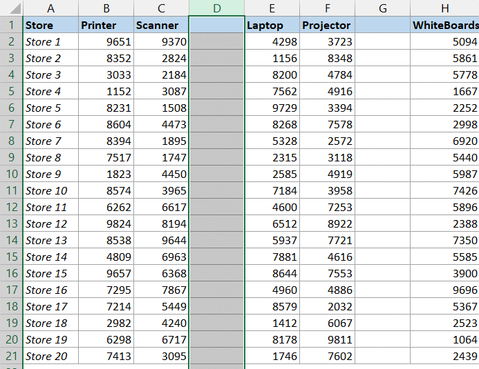

Step 2: Once the blank column is selected, we will right-click on the selection option from the excel sheet.

Step 3: Then, we will click on the 'Delete' option to implement the task.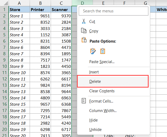

And by performing the above mentioned steps, it would be instantly deleting the entire selected blank column, and after that it will shift the remaining data set to the left direction as well.

Note: It should be noted that we can also select the multiple blank columns in one go by just holding the Control key on our keyboard (or else the Command key if we are making use of the Mac Operating System), and then we can manually click on the column headers of all the available blank columns which we want to select it effectively. And once all the empty columns are selected, we can right-click and after that, click on the Delete option in order to delete all blank columns effectively.

And if we are talking about the biggest drawback of this particular method, is that this method is manual and inefficient; due to which it could be best used for small datasets and not for the larger dataset.

If we are considering the large data set which is incorporated with the huge number of blank columns, then in that case we must need to make use of the other methods, which are discussed below as well.

Deletion of the Blank Columns by making use of the COUNT Function + Sort or the Find and Replace in Microsoft Excel

The Microsoft Excel has an inbuilt functionality which basically allows us to instantly select the available blank cells by the help of the Go To Dialogue box. Still, there is no effective method which can be used to choose only those columns that are empty or blank quickly.

So now we will have to make use of a workaround to identify those columns which are having only the blank cells in them and then proceed to delete these empty columns effectively.

Below we have mentioned the set of the data where we have the sales figures of the various stores for the different items. And as we can see that there are some columns which are empty in the below set of data:

So, now a couple of methods are available in Excel which can be used to remove all blank columns from the above dataset.

By making use of the COUNTA formula with FIND and Replace in Microsoft Excel

With large sets of data, a better and more efficient method that can be used for the purpose of making deletion of all the blank columns by inserting a helper row at the top and then using of a COUNTA formula so to properly identify all the empty columns.

After that, we can make use of the attached helper row to select all the available blank columns quickly and delete them.

Below we have mentioned the data set, in which we have some blank columns we want to remove.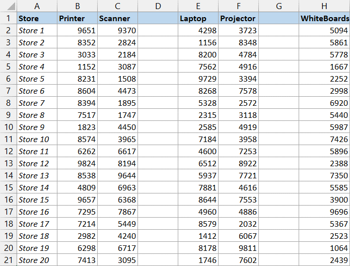

Here are the following steps which can be performed while making use of the COUNTA Function with the helper row:

Step 1: First, we will select the first row of our selected data set by clicking on the row header (as it is the row number in grey given on the left-hand side).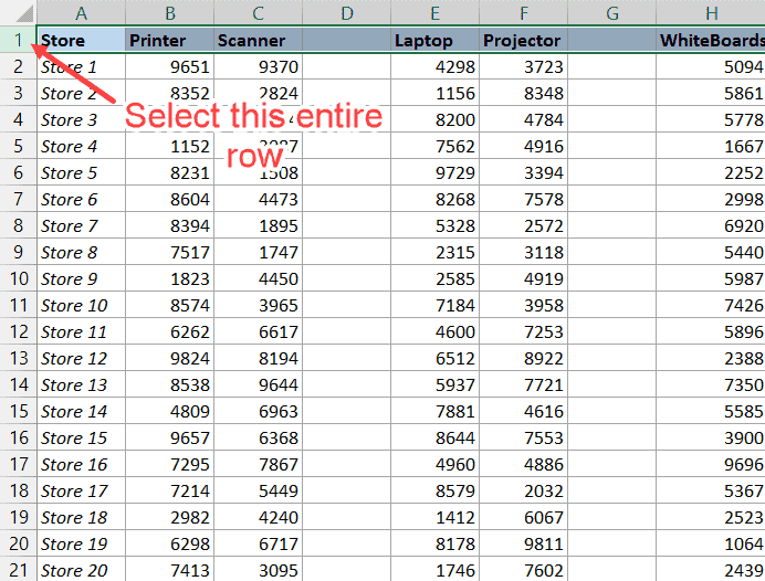

Step 2: In this step, select the entire first row on right-click and then click on the Insert option. As this will insert a new row just above the first row of our data set respectively: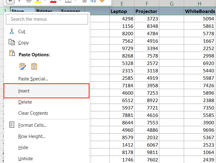

Step 3: And then we will be entering out the below formula in the first respective used cell of the helper row after that we will copy it to all the cells respectively:

And the above used formula primarily makes use of the COUNTA function and then it will be calculating the total number of cells that are not empty in the given specified range.

Besides all this, the used formula will then going to return a value which is greater than zero for all the selected columns which are not empty, as well as zero for any column that is empty:

After that we will be using the IF FUNCTION for the purpose of getting the "Blank" in a cell if the entire column below mentioned is empty and "Not Blank" if it is not empty.

Now, after that we can easily identify all the given empty columns by looking at the values in the mentioned in the helper row. Once we have selected all these cells, we can primarily delete the entire column in one short.

Step to be followed for the purpose of selecting all the empty columns effectively:

Step 1: Firstly, we need to select all the cells in the helper row.

Step 2: After that, we will be holding out the Control key which is there on our keyboard and will press the F key. As this will be opening out the Find and Replace dialogue box, and we can also open the Find and Replace dialogue box by just moving to the 'Home' tab and then clicking on the 'Find & Select' option and clicking on the 'Find' option effectively.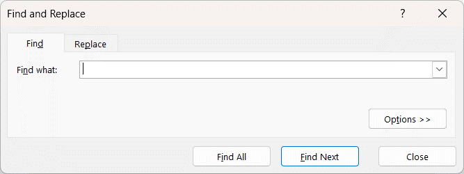

Step 3: Now, in the Find and Replace dialogue box, we will going to enter the text 'Blank' in the 'Find what' field respectively.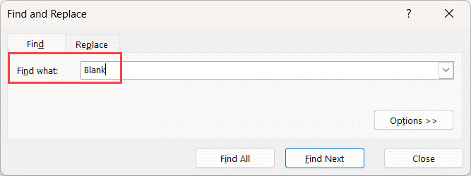

Step 4: After that, we will click on the 'Options' button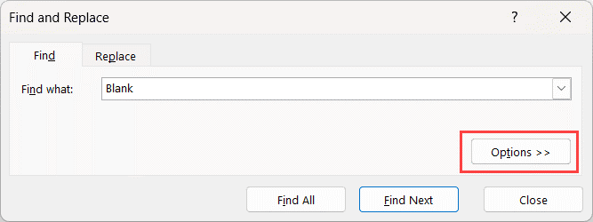

Step 5: Now, in the 'Look in' drop-down menu, we will select 'Values'.

Step 6: After that, we will checking the option 'Match entire cell contents'.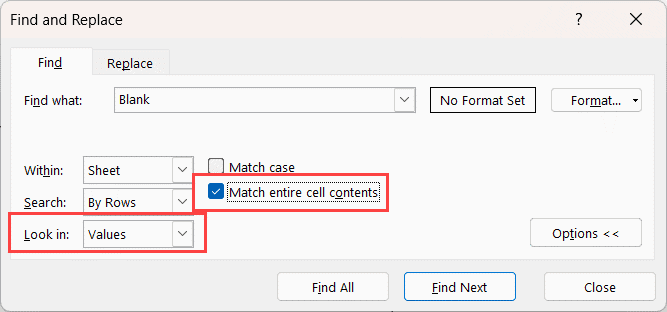

Step 7: In this step, we will be now clicking on the Find All button in order to find and return all the cell references for all the cells which are containing only the text 'Blank'.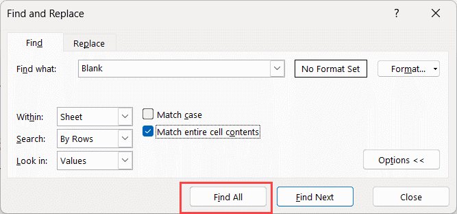

Step 8: Now, we will be holding out the Control key and press the A key to select all the cells given by the Find and Replace options.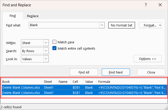

Step 9: Now, we will be right-clicking on any of the cells that have been selected and then clicking on the 'Delete' option.

Step 10: We will select all the 'Entire Column' options in the Delete dialogue box.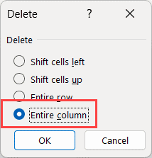

Step 11: After completing the above mentioned step, we will click on the "OK" button respectively.

The above options will instantly delete all the blank columns in our chosen data set.

Important notes:

1. It should be noted that the COUNTA function would only return 0 if all the cells in the column were blank. If there is a header in the given column with no values in it that needs to be removed, then in that case, we need to adjust the respective formula so that the header row should not be used.
   • For example, We can make use of the formula that is:
     =IF (COUNTA (A3:A1048576)=0, "Blank", "Not Blank") in case even blank columns have headers, respectively.
2. Furthermore, the particular columns need to be blank for this formula to work.
   • For example, if there are space characters in the cells present in the blank column, while they might appear to be empty, the COUNTA function would not consider it as blank respectively.

Making use of the COUNTA Formula with the help of the Sort Option in Microsoft Excel

Now we will discuss the other smartest method we can make use too effectively and quickly delete all the empty columns in Microsoft Excel effectively and speedily.

And in this method, we are still making use of the COUNTA function for the purpose of get 'Blank' or 'Not Blank' in the helper row, based on whether the column is empty.

But instead of making use of the Find and Replace dialogue box and we will be making use of the Sort option as well. Below we have the same data set, and we want to remove the blank columns.

Below are the steps which can be used to insert a helper row to identify empty columns:

Step 1: In this, we will select the first row of our data set by clicking on the row header effectively.

Step 2: After that, we will right-click on the Insert option, as this will insert a new row just above the first row of our data set.

Step 3: After then we will move on entering the below formula in the first respective cell of the helper row and copy it down for all the cells in the helper row.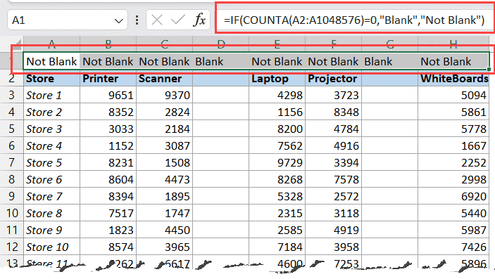

And the above formula would primarily return the text "Blank" in cells where the column below it is empty and "Not Blank" when the column below it is not open.

Now, after that we can easily sort the entire data set by making use of the helper row for the purpose of getting all the blank columns together and all the non-blank columns together.

Below are the steps to perform this efficiently:

Step 1: First, we will select the entire set of the date, including the helper row.

Step 2: After that, we will click on the Data tab present in the excel sheet.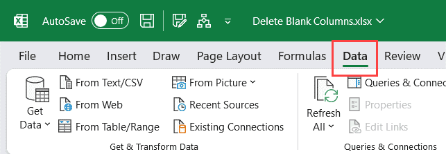

Step 3: Now, in the Sort and Filter group, we will click on the Sort icon, which will open the Sort dialogue box.

Step 4: Then, we will click on the Options button effectively.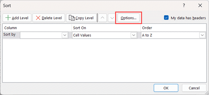

Step 5: Now, in the 'Sort Options' dialogue box, which will open up, we will be clicking on the 'Sort left to right' option effectively; after selecting, we must click on the OK button.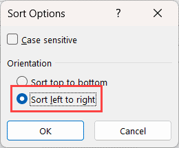

Step 6: In this step, we will click on the 'Sort by' drop-down and then select the 'Row 1' option respectively.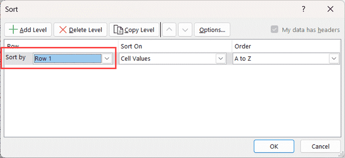

Step 7: After that, we need to keep the Sort Order A to Z. And then finally click on the OK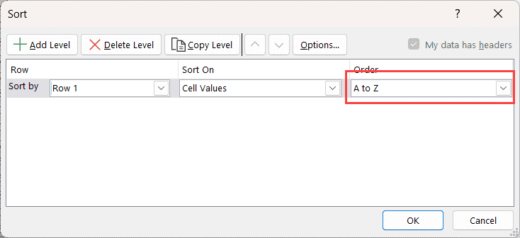

And the above mentioned steps would sort the chosen data that are primarily based on the helper row and also bring all the blank columns together and also the non-blank columns together: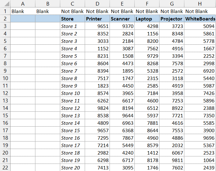

Once we have gathered all the blank columns together, we can select these in one go and then delete them accordingly.

And once we have deleted the blank columns, we can easily remove the helper row from it.

Deletion of the Blank Columns with the help of the VBA (Virtual Basic for Application)

While the above methods, which we have covered in the above section, work great, they require a little bit of a setup by using a helper row.

And suppose we are much more comfortable with VBA (Virtual Basic for Application). In that case, we can find it easier to use than the two helper row methods covered above efficiently.

Code:

The above VBA code usually makes use of the elegant as well as the simple For-Next Loop to go through each column in the Selection; and after that, it will check whether the COUNTA value for all the cells in that column is zero or not respectively.

Moreover, if in a particular case the COUNTA function value is 0, that means the column is empty, and the VBA macro code basically deletes that particular column. Alternatively, if the value of the COUNTA function is seems to be more than 0, then the column is not open and will not be removed in any way.

How to make Use of the above VBA Macro Code in Microsoft Excel?

Now we will be following the below-mentioned steps to make use of the above VBA code to delete an empty column in Excel:

Step 1: First, we will move on to selecting the particular data set with the blank columns which we want to remove.

Step 2: After that, we will click on the Developer Tab in the ribbon.

Step 3: Now, we will be clicking on the Visual Basic icon. As this will be opening the VB editor back end in Microsoft Excel.

Step 4: After that, we will click on the Insert option, which is present under the menu, and then we will click on Module. And after doing this, it will be inserting a new module that would be clearly visible in the Project Explorer pane: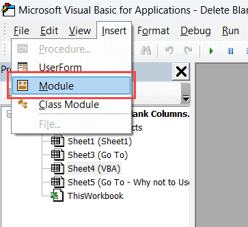

Step 5: Now we need to copy as well as paste the above VBA macro code in the available module code window.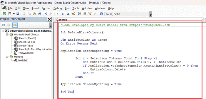

Step 6: And then, to run the macro we will be effectively placing the cursor anywhere in the code and click on the green play icon that are present in the toolbar.

The steps, as mentioned earlier would then instantly run the code and will efficiently remove all the empty columns from the selected data set.

Delete Blank Columns with the help of Go-To Special in Excel

One of the final methods which we want to show is to delete empty Excel columns by just using the Go to Special dialogue box.

As this method is termed to be the fastest method among all the methods that we have discussed in this tutorial, and we need to be more cautious while making use this method when we are dealing with a large data set, it is due to the reason that it can be error-prone and can lead to the deletion of partially blank columns in the excel sheet effectively.

Let us see how this method eventually works in Microsoft Excel.

Below we have a set of some empty columns, and we want to remove these columns.

Steps to be followed:

Step 1: Select the entire set of data.

Step 2: Then, we will press the F5 key from our keyboard to open the Go to a dialogue box.

Step 3: Now, in the Go-To dialogue box which get opens up, in that we will be clicking on the Special button as well.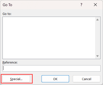

Step 4: Further in the 'Go To Special' dialogue box which opens up on the screen, we will click on the Blanks option.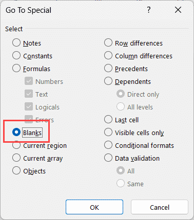

Step 5: And then we will click on the OK button.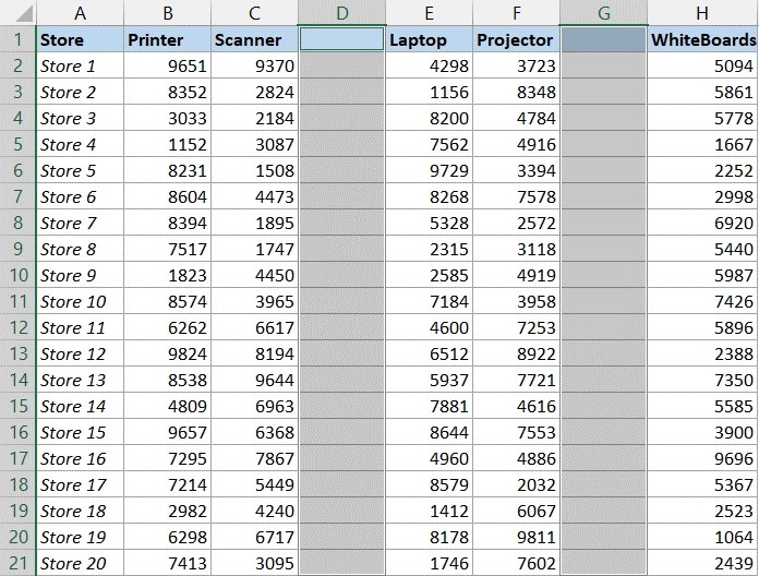

Step 6: And once we have these blank cells selected, we will be right-clicking on any of these blank cells in the empty columns, and will click on the Delete option.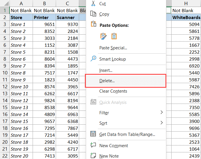

Step 7: This will open the Delete dialogue box where we can choose the Entire column option and click the OK button.