XLOOKUP function in Excel

VLOOKUP and HLOOKUP function has their importance and popularity in Excel. One of the reasons for this popularity is that earlier, there weren't available options whenever the user wanted to look up any value in Excel. For complex formulas, they had to rely upon the INDEX MATCH combination. But not anymore!

With the new version of Excel, i.e., Excel 365 or Excel 2021, you no longer have to choose the above functions - as Microsoft has introduced a more powerful and robust function that overcomes the annoying errors and all the shortcomings of VLOOKUP, the XLOOKUP function.

In many ways, its better than other lookup functions. It can look vertically and horizontally, to the left or above, capturing the ability to search with multiple criteria.

In this tutorial we will covering the following topics:

1. XLOOKUP Function: syntax, parameters, return value
2. Difference between VLOOKUP & XLOOKUP
3. How to implement XLOOKUP in Excel: examples
   • XLOOKUP vertically and horizontally
   • XLOOKUP to the left
   • XLOOKUP with exact and approximate match
   • XLOOKUP with wildcards
   • XLOOKUP last match
   • XLOOKUP and return multiple values (row or column)
   • XLOOKUP with multiple conditions
   • Two-way XLOOKUP
   • If Error XLOOKUP
   • Case-sensitive XLOOKUP
4. XLOOKUP Function not working

XLOOKUP Function: syntax, parameters, return value

"The XLOOKUP function in Excel looks at a range or an array for a given value and returns the corresponding value from another column."

The advantage of using this function is that it can look up both the positions in your table, i.e., vertically and horizontally, and can perform either an exact match (default), an approximate match (the closest data is found), or a wildcard match (using wildcard characters a partial match is found).

Syntax

Parameters

1. Lookup_value (required) - This parameter represents the value to search for in the table.
2. Lookup_array (required) - This parameter represents the table or the range or array where to search.
3. Return_array (required) - It signifies the range or array from where the values will be returned.
4. If_not_found [optional] - This is an optional parameter that represent a value that will be returned if the match is not found. In case you have skipped the parameter, the #N/A error is returned.
5. Match_mode [optional] - This parameter can accept four values depending upon your requirement; if you skip this argument, by default, it takes 0 as its value and returns an exact match.
   • 0 - You can enter this value if you want an exact match.
   • -1 - You can enter this value if you are looking for an exact match or next smaller. It returns the next smaller value, if it not founds and exact match.
   • 1 - You can enter this value if you want to return an exact match or next larger value. If an exact match is not found, the next larger value is returned.
   • 2 - This value represents the wildcard character match.
6. Search_mode [optional] - This parameter helps the user to manage the direction of search. if you skip this argument, by default, it takes 1 as its value and starts the search from first to last position of your array. It can take the following values:
   • 1 - Putting this value will start the search from first to last position of the defined array.
   • -1 - Putting this value will start the search in reverse order i.e., from last to first position.
   • 2 - This value is used if you want to have a binary search where the data is sorted in the ascending order.
   • -2 - This value is used if you want to have a binary search where the data is sorted in the descending order.

Returns

The XLOOKUP function searches a range or an array for predefined value and it returns the related value from another column.

How XLOOKUP Function works?

To understand the working of XLOOKUP function, we will utilize the lookup formula to perform an exact lookup.

For example, we have the names of 5 different salespersons and their monthly sales. Now using XLOOKUP, we have to fetch the sales report of candidates. The name of the person will in cell B1 represents the lookup_value, and now we will look at this value in our lookup_array (A2:A10), and on the basis, of the position, it will return the value from the return array (B2:B10). Our formula becomes: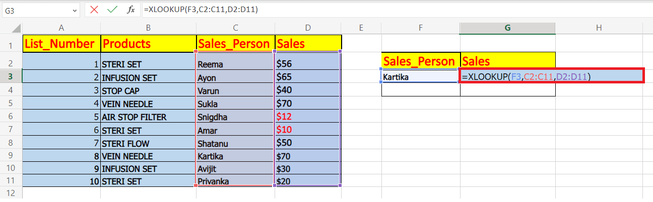

No irritating problems with column index numbers, no sorting required, and no other headaches. Just one single formula and you have your result!

XLOOKUP vs. VLOOKUP

Compared to traditional VLOOKUP, XLOOKUP has many advantages. Below given is a comparison table that lists the differences between XLOOKUP and VLOOKUP:

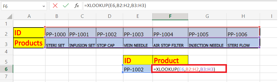
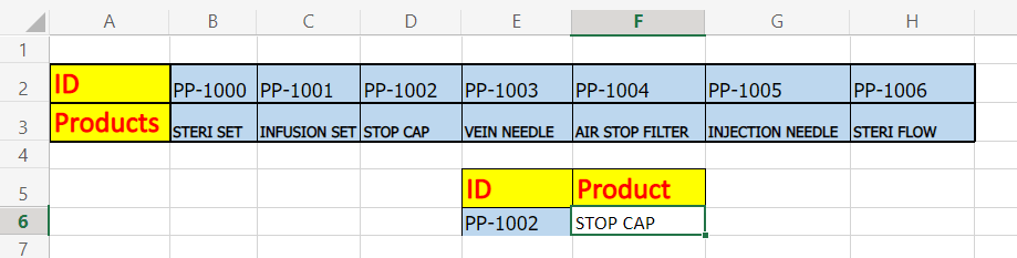
How to implement XLOOKUP in Excel: examples

Example 1: Look up vertically and horizontally

In earlier versions (before Excel 365), if users want to look up vertically or horizontally, they had to implement two functions for different lookup types: VLOOKUP function to look vertically and HLOOKUP to look horizontally.

Luckily, with Excel 2021 or Excel 365, Microsoft introduced XLOOKUP function that is capable to perform both the operations with a single syntax. All you need to do is to supply the respective lookup and return array.

For instance, below is the data sample, given with id, hospital items and their available status.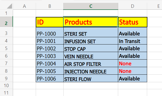

Apply a VLOOKUP:

1. Type the below XLOOKUP formula.

1. Press the enter. It will look for the product from the vertical table.

Applying a HLOOKUP:

1. Type the below XLOOKUP formula. With this, instead of supplying the data arrays vertically we will provide horizontally.

1. Press the enter. It will look for the product from the horizontal table.

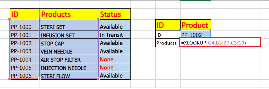
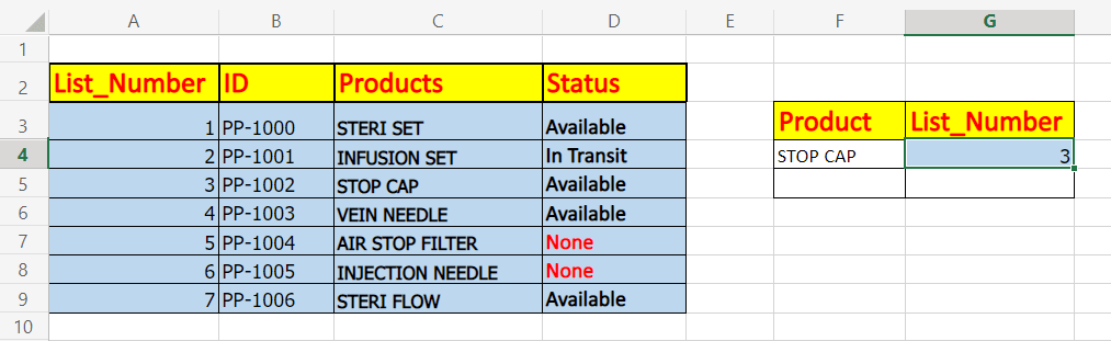
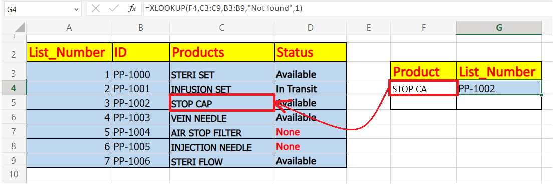
Example 2: Perform left lookup using XLOOKUP

For earlier Excel versions, there wasn't any direct formula to look to the left in your data. You must combine Index and Match functions to apply left lookup in your Excel worksheets. But with the XLOOKUP function, you no longer need to combine Index and match functions. All you need to do is to specify the lookup table, and XLOOKUP will handle the remaining task for you.

For instance, in the above data, we have added another column List_number to the left side. What if we are given the product name and asked to look for the list_number?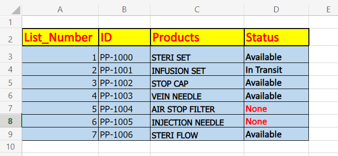

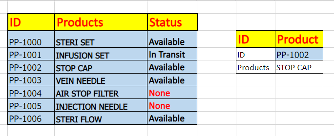
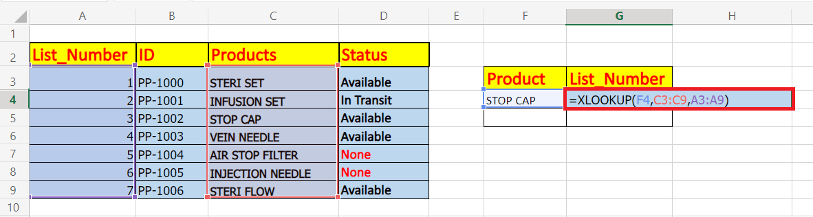
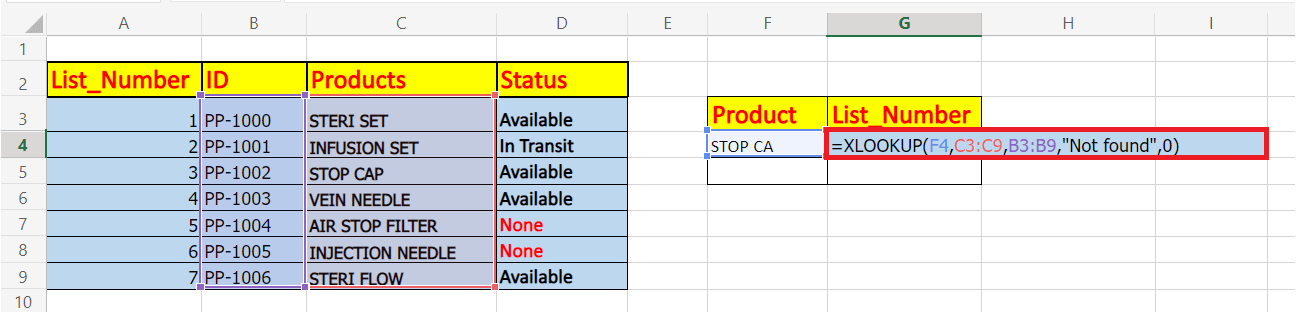
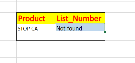
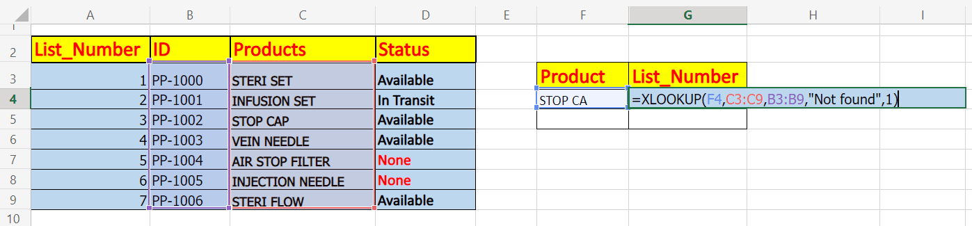
We can use the XLOOKUP function to apply a left lookup in such cases. Follow the below steps to get a left lookup:

1. Type the XLOOKUP function and specify its parameters. The formula will as follows:

1. Press the enter. It will quickly apply the left lookup and will fetch the output from the List_Number table.

Using the same steps, you can implement left lookup horizontally for rows!

Example 3: Perform exact and approximate match

In the beginning, of this tutorial, we have already covered the parameters used in XLOOKUP function. The match_mode parameter controls the match behaviour. It holds four options:

• 0 - Enter this if you want an exact match.
• -1 - Enter this value if you are looking for an exact match or next smaller. It returns the next smaller value, if it not founds and exact match.
• 1 - Enter this value if you want to return an exact match or next larger value. If an exact match is not found, the next larger value is returned.
• 2 - This value represents the wildcard character match.

Exact match XLOOKUP

For most cases, you will use an Exact lookup in Microsoft Excel. Therefore, it's the default attribute, and if you don't pass any value in the match_mode argument, implicitly, it will take 0. Consequently, you can bypass match_mode and provide only the first three required parameters.

1. Type the XLOOKUP function and specify its parameters. The formula will as follows:

1. Press the enter button. It will quickly apply the exact XLOOKUP lookup and fetch the output from the table. Since 'Stop Ca' is not in our table, it will return "Not Found".

Approximate match XLOOKUP

To execute an approximate lookup match, you only need to set the match_mode parameter to -1 or 1, depending on whether you want to return an approximate value for the next smaller or larger data.

For instance, here, we have taken a lookup table that lists the lower bounds of the grades. So, we set match_mode to 1 to search for the next greater value when an exact match is not found:

1. Type the XLOOKUP function and specify its parameters. The formula will as follows:

1. Press the enter button. It will quickly apply the exact XLOOKUP lookup and fetch the output from the table. Since 'Stop Ca' is not in our table, therefore it will look for next greater value and will return the ID number of Stop Cap.

Example 4: To match partial data (wildcards)

XLOOKUP provides the option to execute a partial match lookup. All you need to do is to set the match_mode parameter to 2. Primarily, most of the users prefer to use the following wildcard characters:

1. An asterisk (*) - This wildcard character is used to define the sequence of characters.
2. A question mark (?) - This wildcard character is used to define any single character.

Let's implement the partial match using a real-time example.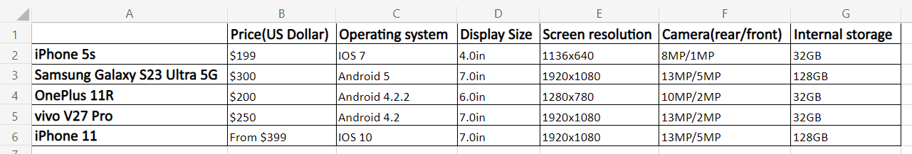

The above table lists phones' features, storage, price, display, etc. You are interested in the price of a certain smartphone. The only problem here is you only know about the phone name, not the complete model name, exactly as it appears in column A. The solution is to enter the phone name and replace the front and back characters with wildcards.

Let's suppose we want to fetch information about the price of Samsung formula, we will incorporate the following formula with wildcard characters and will set the match_mode argument to 2: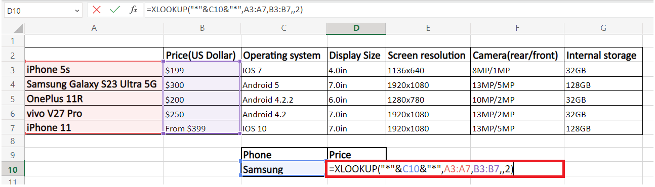

The above formula will return the pricing after partially matching Samsung from the table: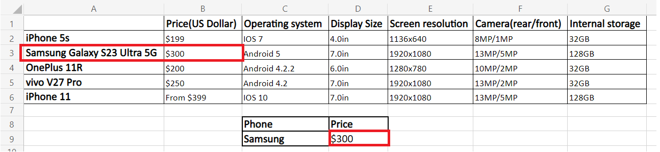

Note: Instead of a cell reference, you can also directly pass the phone name between the double inverted commas (" ").

Example 5: Work in Reverse order to get last occurrence

Sometimes, your lookup table contains multiple instances of the lookup value. By default, the XLOOKUP formula fetches the matched output of the first occurrence of the lookup value. But what if you want to return to the last match? To have it done, all you need to do is to set the Xlookup formula to search in the reverse direction.

You can control the order of the search by the 6th parameter named search_mode:

• 1 (default value)- Enter this if you want to set your search from first to last value.
• -1 - Use this if you want to set your search in reverse order or want to fetch the last to first value.

For example, let's implement the XLOOKUP formula to return the last sale value of the product 'STERI SET'. Unlike the above formulas, we put together the first three required arguments (E3 for lookup_value argument, B2:B11 for lookup_array, and C2:D11 for return_array argument), and this time will set the 5th parameter to -1.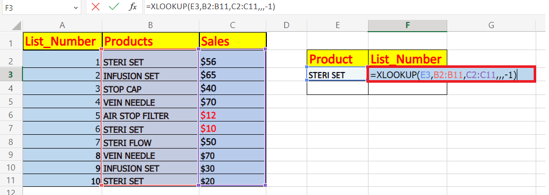

As a result, it will search for the last occurrence of the lookup_value "STERI SET" and will return the lowest pricing.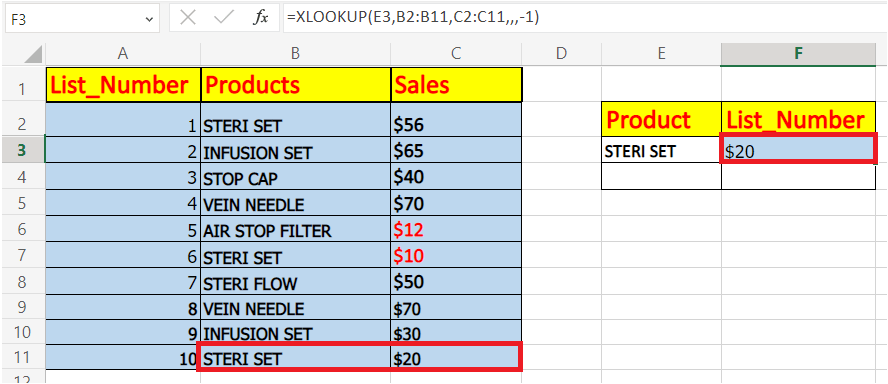

Example 6: Return multiple columns or rows

Do you know the XLOOKUP function is not limited to returning a single value? Using this formula, you can return more than one value associated with the same lookup_value. And to implement, you need to enter only the first three required arguments without any additional manipulations!

As an example, suppose from the above table (Data of Smartphones) you are asked to fetch all the details of a specific phone. The formula to implement this is very simple. Instead of a single column, what you need to do is supply the entire range (B1: G6) for the return_array parameter: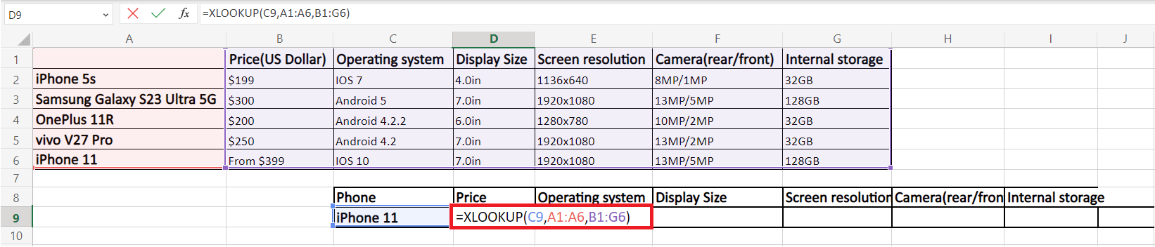

All you need to do is to enter the formula, and Ms. Excel will automatically spill the output into adjacent blank cells. In our case, it has returned all six columns. Refer to the following output: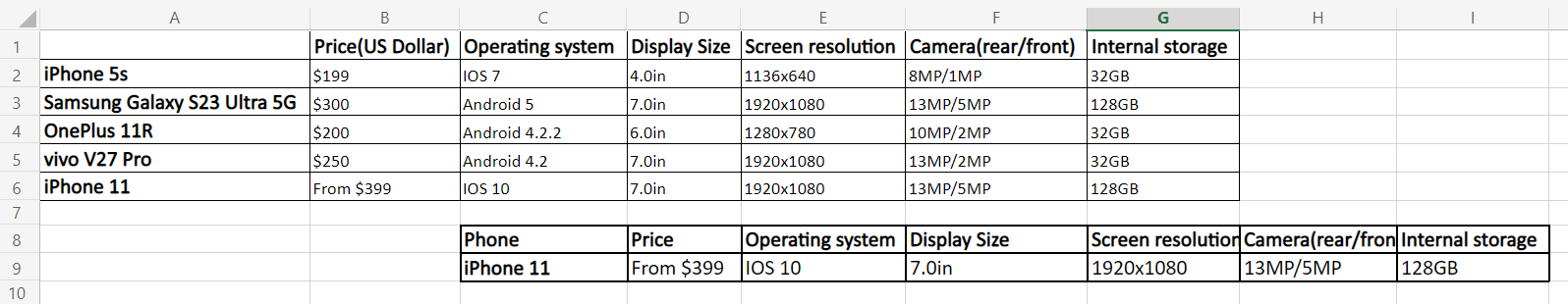

Using the Transpose function, you can also return the above output vertically in a column. Nesting the XLOOKUP into Transpose will automatically flip the array vertically.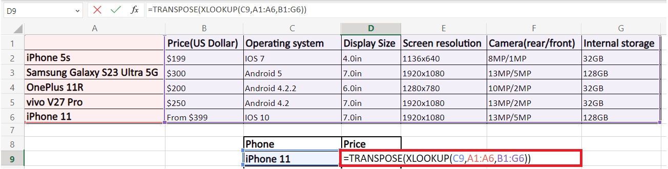

You will have the following output: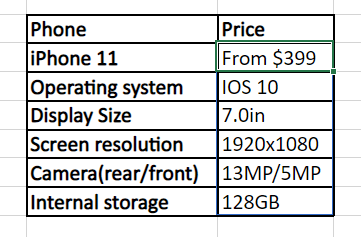

Note: Before using this formula, ensure you have enough empty cells towards the right or downside of the formula cell. Because multiple values are adjusted into neighboring cells, if Excel finds any data, it will return a #SPILL! error.

Example 7: XLOOKUP Multiple Criteria

One more amazing feature of XLOOKUP is that it handles arrays natively. Because of this feature it can easily work with multiple criteria directly in the lookup_array parameter. Follow the below syntax for multiple criteria:

The output of each criteria is an array of either TRUE or FALSE values. But since we are multiplying the arrays, the TRUE or FALSE Boolean values get converted into 1 and 0, respectively, generating the resultant lookup array. As per the basic maths rule, if you multiply anything with 0, the output will always be zero; therefore, in the lookup table, only the items that meet all the criteria are represented by 1.

You can check in the below table that we are given three criteria to check. Based on those criteria we have figure out the Sales from E2:E11 (return_array).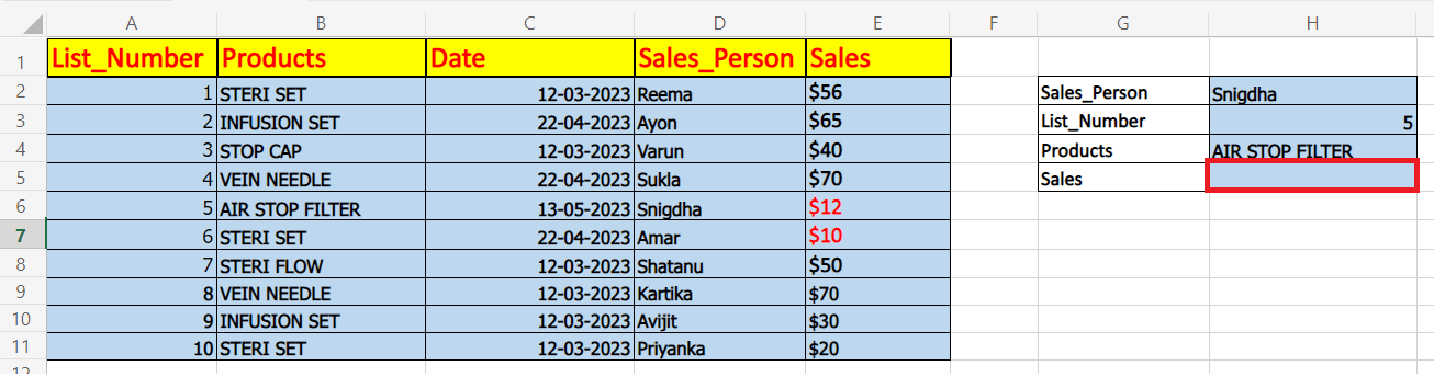

We will be applying three criteria's which are as follows:

1. Criteria1 (sales_person) = H2
2. Criteria2 (List_number) = H3
3. Criteria3 (Products) = H4

The formula takes this shape: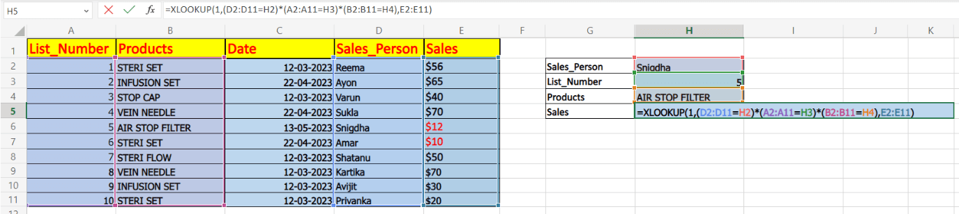

As a result, the XLOOKUP function will process all the criteria, and if each criterion is fulfilled, it will look for the output from the return array.

Example 8: Double (Two Way) XLOOKUP

Two-way or Double lookups are commonly used to find the intersection value of a given row and column. To your surprise, Excel XLOOKUP can do that too! All it requires is to nest XLOOKUP into another, and you will have the following syntax:

For this example, we are given Sales_Report of three months i.e., S1, S2, S3. Here, we will find the sales report of a particular salesperson within S3 quarter. To solve the problem, we will use two-way Xlookup with the following formula: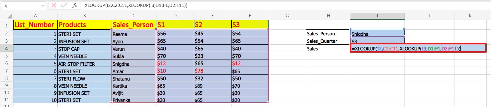

Example 9: Case-sensitive XLOOKUP

In the above examples, you might have noticed that the XLOOKUP function treats the lowercase and uppercase letters as same. By default, this function is case-sensitive. To make XLOOKUP case-sensitive, we will replace the parameter lookup_array with the EXACT function. Use the following syntax:

As the name suggests, the role of the EXACT function is to compare the given lookup value to each value in the array; if it gets matched (including the letter case), it returns TRUE. Now, XLOOKUP matches its lookup value with its lookup array, and if both are TRUE, it searches the TRUE for the given array and returns the match from the return array.

Let's suppose we want to fetch Sales data of product STERI SET with a Case-sensitive match, we will be using the following formula: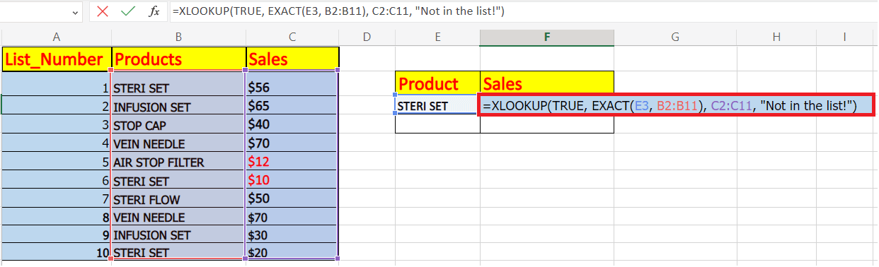

Since it found an exact found, it will return the sales value from the return array,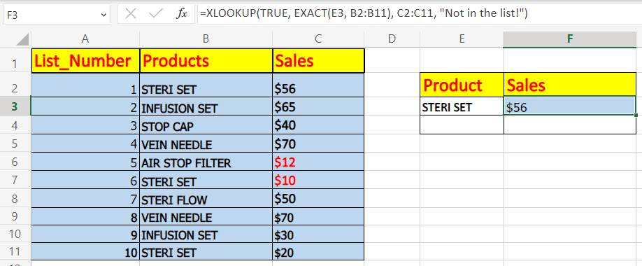

Note. If your lookup array contains two or more same data, the XLOOKUP function will return the first match value.

Example 10: If Error XLOOKUP

The XLOOKUP function returns the #N/A error if the lookup value is not found. While using the formula professionally, the #N/A error doesn't look good and could even be confusing for many intermediate Excel users. Therefore, catching the error and writing a user-friendly note are always advised.

For example, let's consider a case when the match is not found.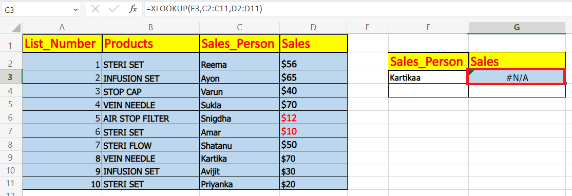

As a result, you got an #N/A error. To replace the error with your customized message, you need to add a text in the fourth argument.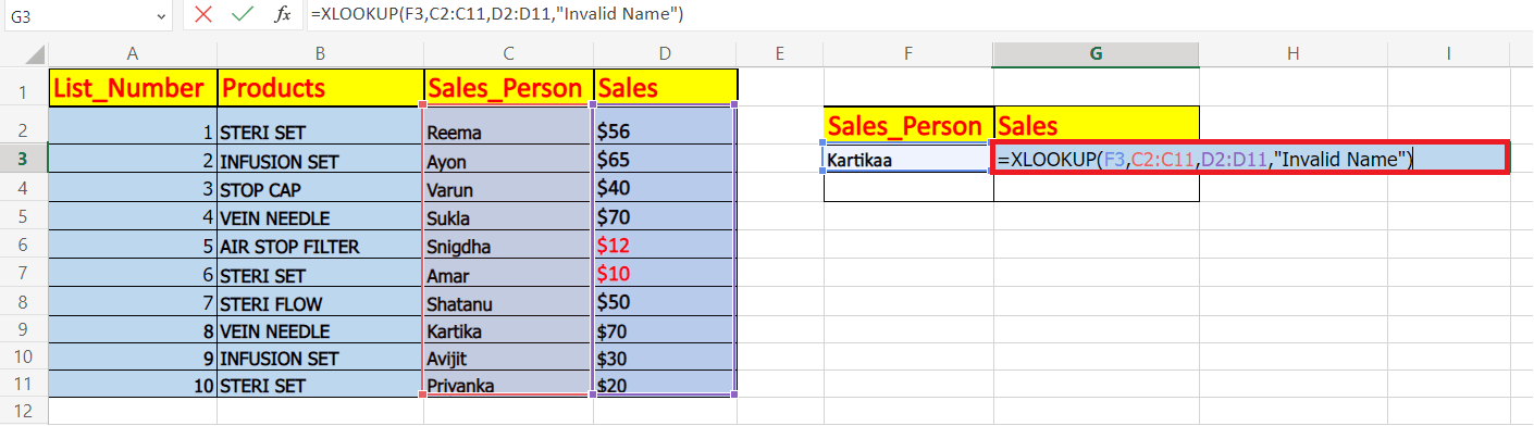

For instance, if someone inputs an invalid product name, our formula will return "Invalid name" message.

XLOOKUP Function not working

Many times your Excel XLOOKUP formula does work properly, and often it ends up returning an error. It mostly occurs because of one of the following reasons:

1. You are using XLOOKUP with previous Excel version.

The only catch with the XLOOKUP function is that it is not backward compatible, and is only available in Excel for Microsoft 365 and Excel 2021 and cannot be used in earlier versions.

2. Excel XLOOKUP returns wrong output

Sometimes, this Excel function may return the wrong output. The common reason is that you have put the wrong data values, or the return_array range might have shifted while copying the formula down the cells. You can prevent this by using absolute cell references (for example, $A$1:$A$20). in both ranges, and it will lock both the array ranges and return the correct output.

3. XLOOKUP function returns #N/A error

The XLOOKUP function returns an #N/A error if it cannot find the lookup value from the lookup table. However, you can exchange the error with your customized message.

4. XLOOKUP function returns #VALUE error

A #VALUE! error occurs if the lookup and return arrays have incompatible dimensions. For example, if in the parameters you have supplied a lookup_array horizontally and want to return the values for a vertical return_array.

5. XLOOKUP function returns #REF error

This function throws a #REF! error when looking up for data between two different workbooks, and out of which one of the workbooks is closed. To fix the error, simply open both files.