Deep Learning Definition

Deep learning belongs to a larger group of machine learning techniques that are built on artificial neural networks and representation learning. The three types of learning are supervised, semi-supervised, and unsupervised.

Deep-learning architectures like deep neural networks, deep belief networks, deep reinforcement learning, recurrent neural networks, convolutional neural networks, and transformers have been used in fields like computer vision, speech recognition, natural language processing, machine translation, bioinformatics, drug design, medical image analysis, climate science, material inspection, and board game programmes. These applications have led to results that are on par with and i.

Artificial neural networks (ANNs) were developed as a result of biological systems' dispersed communication and information processing nodes. Biological brains and ANNs differ in a number of ways. The biological brain of the majority of living species is dynamic (plastic) and analogue, in contrast to artificial neural networks, which tend to be static and symbolic.

The usage of several network layers is indicated by the term "deep" in deep learning. Early research shown that a network with one hidden layer of unbounded breadth and a nonpolynomial activation function can be a universal classifier but a linear perceptron cannot. A contemporary form known as deep learning is focused on an infinite number of layers with bounded sizes, allowing for practical application and optimised implementation while maintaining theoretical universality under benign circumstances. For the sake of efficiency, trainability and understandability deep learning also permits the layers to be diverse and to depart significantly from biologically inspired connectionist models.

Definition:

Deep learning is a category of machine learning algorithms[8]: 199-200 that employs numerous layers to gradually extract higher-level information from the input. As an illustration, in image processing, lower layers may recognise borders, whereas higher layers may identify things important to humans, such as numbers, letters, or faces.

A different way to look at deep learning is to think of it as the "computerization" or "automation" of human learning processes from a source, like an image of dogs, to an item that has been learnt (dogs). So it seems sense that there is a concept known as "deeper" or "deepest" learning. When learning from a source to a final learnt object is totally automated, that is considered to be the deepest learning. The phrase "deeper learning" thus refers to a blended learning process that involves first learning by humans from a source to a learned semi-object, then learning by computers from the semi-object to the final learnt object.

Overview:

The majority of contemporary deep learning models are built on artificial neural networks, specifically convolutional neural networks (CNNs), though they can also incorporate propositional formulas or latent variables organised layer-wise in deep generative models, like the nodes in deep belief networks and deep Boltzmann machines.

In deep learning, each level picks up the ability to express its input data in a composite representation that is a little more abstract. In an image recognition application, the initial input could be a matrix of pixels; the first representational layer could abstract the pixels and encode edges; the second layer could compose and encode arrangements of edges; the third layer could encode a nose and eyes; and the fourth layer could recognise that the image contains a face. What's more, a deep learning process may figure out for itself which traits are most suited for which level. This does not negate the necessity for manual adjustment; for instance, adjusting the number of layers and the size of the layers can offer various levels of abstraction.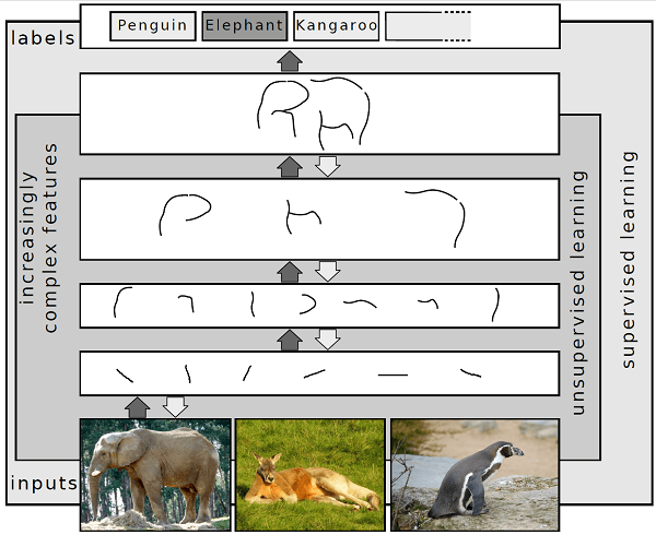

The term "deep" in "deep learning" refers to the quantity of layers through which the data is changed. Deep learning systems specifically have a significant credit assignment path (CAP) depth. The series of transformations leading from input to output makes up the CAP. CAPs describe the relationships between input and output that might be causative. For a feedforward neural network, the number of hidden layers plus one (because the output layer is also parameterized) determines the depth of the CAPs. The CAP depth is conceivably limitless for recurrent neural networks, where a signal may pass through a layer more than once. Although there isn't a depth cutoff that distinguishes deep learning from shallow learning in all cases, most researchers concur that deep learning requires CAP depths greater than 2. It has been demonstrated that CAP of depth 2 is a universal approximator in the sense that it can simulate any function. Beyond that, adding layers does not improve the network's capacity to approximate functions. Extra layers aid in effectively learning the features since deep models (CAP > 2) are able to extract better features than shallow models.

An aggressive layer-by-layer approach can be used to create deep learning structures. Disentangling these abstractions and identifying the attributes that enhance performance are made possible by deep learning.

Deep learning techniques reduce the need for feature engineering while performing supervised learning tasks by converting the data into compact intermediate representations (similar to principal components) and generating layered structures that minimise redundant representations.

To do unsupervised learning tasks, deep learning algorithms can be used. Given that there are more unlabeled data than labelled data, this is a significant advantage. Deep belief networks are an instance of a deep structure that can be learned unsupervised.

Interpretations:

Deep neural networks are typically explained in terms of probabilistic inference or the universal approximation theorem.

A feedforward neural network with a single hidden layer of finite size can estimate continuous functions, according to the standard universal approximation theorem. George Cybenko published the first evidence for sigmoid activation functions in 1989, and Kurt Hornik generalised it to feed-forward multi-layer structures in 1991. Additionally, recent research demonstrated that universal approximation also applies to non-bounded activation functions, such as the rectified linear unit of Kunihiko Fukushima.

The capacity of deep neural network networks with bounded width but unrestricted depth is addressed by the universal approximation theory for deep neural networks. According to Lu et al.'s research, if the width of a deep neural network with ReLU activation is strictly greater than the input dimension, the network can approximate any Lebesgue integrable function; however, if the width is smaller than or equal to the input dimension, a deep neural network is not a universal approximator.

From the study of machine learning comes the probabilistic interpretation. It includes the concept of inference as well as the training and testing optimisation techniques, which are connected to fitting and generalisation, respectively. A cumulative distribution function is explicitly taken into account by the probabilistic interpretation of the activation nonlinearity. In neural networks, dropout was first introduced as a regularizer as a result of the probabilistic interpretation. Researchers like Hopfield, Widrow, and Narendra presented the probabilistic interpretation, and surveys like the one by Bishop helped make it widespread.

History:

Recurrent neural networks (RNNs) and feedforward neural networks (FNNs) are the two varieties of neural networks. Cycles exist in the connection structure of RNNs but not FNNs. The Ising model, which is essentially a non-learning RNN architecture made up of threshold elements that resemble neurons, was developed and studied by Wilhelm Lenz and Ernst Ising in the 1920s. This architecture was made adaptable in 1972 by Shun'ichi Amari. John Hopfield made his learning RNN well-known in 1982. Speech recognition and language processing now heavily rely on RNNs. In his book from 1962, Frank Rosenblatt introduced the multilayer perceptron (MLP), which had three layers: an input layer, a hidden layer with randomised weights that did not learn, and an output layer. According to Charles Tappert, Rosenblatt developed and investigated all of the fundamental components of the deep learning systems used today. This was hardly deep learning, though, as only the output layer contained learning connections. It was a machine that was later referred to as an extreme learner.

In 1967, Alexey Ivakhnenko and Lapa published the first generic, functional learning algorithm for supervised, deep, feedforward, multilayer perceptrons. A deep network with eight layers that was trained using the group approach of data handling was described in a 1971 article. Using stochastic gradient descent, Shun'ichi Amari developed the first multilayer perceptron for deep learning in 1967. An MLP with five layers and two changeable levels that developed internal representations to categorise non-linearly separable pattern classes was used in computer studies by Amari's student Saito.

The reverse method of automated differentiation of discrete connected networks of nested differentiable functions was published in 1970 by Seppo Linnainmaa. Backpropagation was coined to describe this. It is an effective application to networks of differentiable nodes of the chain rule derived by Gottfried Wilhelm Leibniz in 1673. Although Henry J. Kelley had a continuous antecedent of backpropagation in the context of control theory as early as 1960, Rosenblatt actually coined the phrase "back-propagating errors" in 1962, but he had no idea how to put it into practise.

Paul Werbos first introduced backpropagation to MLPs in the manner that is now considered standard in 1982. An experimental investigation of the approach was published in 1985 by David E. Rumelhart et al.

Beginning with Kunihiko Fukushima's Neocognitron, which he unveiled in 1980, deep learning architectures for convolutional neural networks (CNNs) featuring convolutional layers and downsampling layers were developed. He also created the ReLU (rectified linear unit) activation function in 1969. The rectifier is now the most widely used activation function for CNNs and deep learning in general. CNNs have developed into a crucial computer vision technique.

In the context of Boolean threshold neurons, Igor Aizenberg and colleagues introduced the term "Deep Learning" to the machine learning community in 1986, and Rina Dechter did the same for artificial neural networks in 2000.

The backpropagation algorithm was used by Wei Zhang et al. in 1988 to recognise letters using a convolutional neural network (a convolutional Neocognitron with convolutional links between the image feature layers and the final fully connected layer). Additionally, they suggested using an optical computing system in conjunction with CNN. To identify handwritten ZIP codes on mail, Yann LeCun et al. used backpropagation on a CNN in 1989. The algorithm worked, although the training process took three days. The last completely linked layer was then removed by Wei Zhang, et al., who then adjusted the model and used it for breast cancer diagnosis in mammograms in 1994 as well as object segmentation in medical images in 1991. Several banks have used LeNet-5 (1998), a 7-level CNN that categorises digits, to identify handwritten numbers on checks that have been digitally enhanced into 32x32 pixel images.

Backpropagation did not perform well for deep learning in the 1980s when there were lengthy credit assignment channels. Juergen Schmidhuber (1992) presented a hierarchy of RNNs that were pre-trained one level at a time by self-supervised learning to solve this issue. To learn internal representations across a range of self-organizing time scales, it employs predictive coding. This has the potential to greatly aid downstream deep learning. By condensing a higher level chunker network into a lower level automatizer network, the RNN hierarchy can be broken down into a single RNN. A deep learning challenge with a depth of more than 1000 was solved in 1993 using a chunker.

A RNN substitute known as a linear Transformer or a Transformer with linearized self-attention was also reported by Juergen Schmidhuber in 1992, with the exception of a normalisation operator. A slow feedforward neural network learns by gradient descent to control the fast weights of another neural network using the outer products of self-generated activation patterns FROM and TO (which are now dubbed key and value for self-attention). This method teaches internal spotlights of attention. An application of this quick weight attention mapping is made to a query pattern.

Ashish Vaswani et al. first described the contemporary Transformer in their 2017 paper "Attention Is All You Need." This is coupled with a projection matrix, a softmax operator, and both. Transformers are more and more popular as the natural language processing model. The GPT-4, BERT, and ChatGPT are just a few examples of contemporary large language models that make use of it. Transformers are also being employed more and more in computer vision.

Juergen Schmidhuber also released adversarial neural networks in 1991, which compete against one another in the manner of a zero-sum game in which the winner loses to the loser. A probability distribution over output patterns is modelled by the first network, which is a generative model. The second network uses gradient descent to learn to foretell how the environment will respond to these patterns. It was referred to as "artificial curiosity." This idea was applied by Ian Goodfellow and colleagues in 2014 in a generative adversarial network (GAN). If the output of the first network is included in the specified set, the environmental response in this case will be either 1 or 0. This can be used to make deep fakes that are realistic. Nvidia's StyleGAN (2018), which is based on the Progressive GAN by Tero Karras et al., produces excellent image quality. In this case, the GAN generator is pyramidally scaled up from tiny to gigantic.

According to Sepp Hochreiter's supervisor Schmidhuber, his diploma thesis from 1991 is "one of the most significant records in the history of machine learning." In addition to putting the neural history compressor to the test, it also located and examined the vanishing gradient issue. Recurrent residual connections were suggested by Hochreiter as a solution to this issue. Long short-term memory (LSTM), a deep learning technique, was developed as a result and first published in 1997.

Recurrent neural networks with long credit assignment routes that require memories of past events that occurred thousands of discrete time steps ago can learn "very deep learning" tasks using LSTMs. 1999 saw the release of the "vanilla LSTM" with forget gate by Felix Gers, Schmidhuber, and Fred Cummins. The most frequently used neural network of the 20th century is LSTM. The Highway network, a feedforward neural network with hundreds of layers and far more depth than earlier networks, was developed in 2015 by Rupesh Kumar Srivastava, Klaus Greff, and Schmidhuber using LSTM principles. Seven months later, Kaiming He, Xiangyu Zhang, Shaoqing Ren, and Jian Sun won the ImageNet 2015 contest using a form of the Highway network called the Residual neural network that is open-gated or gateless. The most often referenced neural network of the twenty-first century is now this one.

In 1994, André de Carvalho, Mike Fairhurst, and David Bisset published the experimental findings of a multi-layer boolean neural network, also referred to as a weightless neural network. This network was made up of three layers of self-organizing feature extraction neural network module (SOFT), followed by multiple layers of classification neural network module (GSN), both of which were trained independently. With respect to the preceding layer, the feature extraction module's subsequent layers extracted features that were more complicated.

Brendan Frey showed in 1995 that the wake-sleep method, which he co-developed with Peter Dayan and Hinton, could be used to train a network with six fully linked layers and several hundred hidden units over the course of two days. Since 1997, Sven Behnke has added lateral and backward connections to the feed-forward hierarchical convolutional technique in the Neural Abstraction Pyramid to more easily incorporate context into decisions and iteratively clear up local ambiguities.

In the 1990s and 2000s, simpler models with task-specific handcrafted features, such as Gabor filters and support vector machines (SVMs), were a preferred option due to the computationally expensive nature of artificial neural networks (ANNs) and the lack of knowledge about the biological network wiring of the brain at the time.

For many years, recurrent nets and other ANNs with shallow and deep learning have both been investigated for use in voice recognition. These techniques have never been able to match the performance of non-uniform internal-handcrafting Gaussian mixture model/Hidden Markov model (GMM-HMM) technology built on generative models of speech that have undergone discriminative training. The weak temporal correlation structure and gradient decrease in neural predictive models have been identified as major challenges. Insufficient training data and inadequate processing capacity were further challenges.

In order to focus on generative modelling, the majority of voice recognition researchers abandoned neural nets. A notable exception occurred in the late 1990s at SRI International. Deep neural networks for speech and speaker recognition were explored by SRI with funding from the NSA and DARPA of the US government. In the 1998 National Institute of Standards and Technology Speaker Recognition evaluation, the speaker identification team led by Larry Heck reported significant success with deep neural networks in speech processing. As the first significant industrial application of deep learning, the SRI deep neural network was subsequently implemented in the Nuance Verifier.

In the architecture of the deep autoencoder on the "raw" spectrogram or linear filter-bank features in the late 1990s, the principle of elevating "raw" features over hand-crafted optimisation was first successfully explored, demonstrating its superiority over the Mel-Cepstral features that contain stages of fixed transformation from spectrograms. Waveforms, the basic building blocks of speech, later yielded outstanding outcomes on a broader scale.

LSTM replaced speech recognition in that process. On several tests, LSTM began to match up well with conventional speech recognizers in 2003. In stacks of LSTM RNNs, it was integrated with connectionist temporal classification (CTC) by Alex Graves, Santiago Fernández, Faustino Gomez, and Schmidhuber in 2006. According to reports, in 2015, Google's voice recognition had a significant performance increase of 49% thanks to CTC-trained LSTM, which they made accessible through Google Voice Search.

According to Yann LeCun, CNNs started processing 10% to 20% of all US checks made in the early 2000s, when deep learning first started to have an impact on the business world. Large-scale deep learning speech recognition applications in industry first appeared around 2010.

Geoff Hinton, Ruslan Salakhutdinov, Osindero, and Teh demonstrated in publications from 2006 how a multi-layered feedforward neural network can be efficiently pre-trained one layer at a time by treating each layer as an unsupervised restricted Boltzmann machine and then fine-tuning it using supervised backpropagation. Developing learning for deep belief nets was discussed in the publications.

The 2009 NIPS Workshop on Deep Learning for Speech Recognition was inspired by the shortcomings of deep generative models of speech as well as the potential for deep neural networks (DNNs) to be used in practical applications with better hardware and larger data sets. It was thought that the primary issues with neural nets might be solved by pre-training DNNs using generative models of deep belief nets (DBN). However, it was found that using DNNs with large, context-dependent output layers for simple backpropagation instead of pre-training resulted in error rates dramatically lower than then-state-of-the-art Gaussian mixture model (GMM)/Hidden Markov Model (HMM) as well as than more-advanced generative model-based systems.

Technical insights regarding how to incorporate deep learning into the current, very effective, run-time speech decoding system used by all major speech recognition systems are provided by the nature of the recognition errors created by the two types of systems, which were distinctively different. Early industrial interest in deep learning for speech recognition was sparked by analysis conducted in 2009-2010 that compared the GMM (and other generative speech models) with DNN models. Between discriminative DNNs and generative models, the study was conducted with performance that was equivalent (less than 1.5% error rate). In 2010, researchers applied deep learning from TIMIT to recognise speech with a vast vocabulary by adopting extensive output layers of the DNN based on context-dependent HMM states created by decision trees.

Modern computer vision and automatic speech recognition (ASR) systems, in particular, incorporate deep learning as part of their architecture. Results on many large-vocabulary voice recognition tasks, as well as on widely used evaluation sets like TIMIT (ASR) and MNIST (image classification), have gradually increased. Convolutional neural networks (CNNs) were replaced by CTC for LSTM in place of convolutional neural networks (ASR), however they perform better in computer vision.

Deep learning is now more popular than ever thanks to hardware improvements. Nvidia was a part of what was referred to as the "big bang" of deep learning in 2009, "as deep-learning neural networks were trained with Nvidia graphics processing units (GPUs)." In that year, Andrew Ng discovered that GPUs could speed up deep-learning systems by a factor of roughly 100. GPUs are especially well adapted for the matrix/vector computations needed for machine learning. By orders of magnitude, GPUs accelerate training methods, cutting down on their weeks-long runtimes. Deep learning models can be processed effectively using specialised technology and algorithm optimisations, among other things.

The Revolution in Deep Learning:

In machine learning competitions in the late 2000s, deep learning began to perform better than other approaches. As the first RNN to triumph in pattern recognition competitions, a long short-term memory trained through connectionist temporal classification (Alex Graves, Santiago Fernández, Faustino Gomez, and Juergen Schmidhuber, 2006) won three competitions in connected handwriting recognition in 2009. Later, for speech recognition on smartphones, Google employed LSTM that had been CTC-trained.

Between 2011 and 2012, there were significant effects on image or object recognition. Although CNNs trained using backpropagation had been around for years and CNNs had been implemented on GPUs for many years, faster CNN implementations on GPUs were required to advance computer vision. Dan Ciresan, Ueli Meier, Jonathan Masci, Luca Maria Gambardella, and Juergen Schmidhuber's DanNet beat out conventional techniques by a factor of three in a visual pattern recognition competition in 2011. This was the first time superhuman performance had been attained. In May 2012, DanNet triumphed in the ISBI image segmentation competition after winning the ICDAR Chinese handwriting competition in 2011.

A study by Ciresan et al. at the prestigious conference CVPR in June 2012 demonstrated how max-pooling CNNs on GPU may significantly improve several vision benchmark records, a significant change from the state of affairs up until that point in which CNNs were not often discussed in computer vision conferences. The ICPR competition on the analysis of huge medical images for cancer detection was also won by DanNet in September 2012, and the MICCAI Grand Challenge on the same issue was won by the company the following year. Similar AlexNet developed by Alex Krizhevsky, Ilya Sutskever, and Geoffrey Hinton triumphed over shallow machine learning approaches to win the large-scale ImageNet competition in October 2012.

Following a similar pattern in massive voice recognition, the VGG-16 network developed by Karen Simonyan and Andrew Zisserman considerably decreased the error rate and won the ImageNet 2014 competition.

After that, image classification was expanded to include the more difficult duty of creating captions for images, frequently using a mix of CNNs and LSTMs.

Using multi-task deep neural networks to foretell the biomolecular target of one medicine, a team lead by George E. Dahl won the "Merck Molecular Activity Challenge" in 2012. The "Tox21 Data Challenge" of the NIH, FDA, and NCATS was won in 2014 by Sepp Hochreiter's team, who employed deep learning to identify off-target and harmful effects of environmental chemicals in foods, home products, and medications.

A "deep learning revolution" that has altered the AI sector was described by Roger Parloff in 2016.

The Turing Award was given to Yoshua Bengio, Geoffrey Hinton, and Yann LeCun in March 2019 in recognition of their conceptual and technical innovations that make deep neural networks an essential part of computing.

Networks of Neurons:

Computer systems called artificial neural networks (ANNs) or connectionist systems are modelled after the biological neural networks seen in animal brains. These systems, which typically lack task-specific programming, learn (gradually get better at doing) tasks by taking into account examples. For instance, in image recognition, they might study sample pictures that have been manually labelled as "cat" or "no cat" and then analyse them, utilising the results of the analysis to find cats in other pictures. Utilising rule-based programming, they have been most useful in applications that are challenging to express with a conventional computer algorithm.

A network of interconnected artificial neurons-which are comparable to biological neurons in a biological brain-forms the foundation of an ANN. A signal can be sent from one neuron to another at any point where two neurons join (synapse). In order to signal downstream neurons attached to it, the receiving (postsynaptic) neuron can process the signal(s). In general, real numbers between 0 and 1 are used to indicate the state of neurons, which can range from '0' to '1'. Additionally, as learning progresses, the weight of neurons and synapses may change, affecting the strength of the signal they send to downstream neurons.

Layers are the typical structure for neurons. Alterations to the inputs of several layers may take various forms. Signals may pass through the layers more than once as they move from the first (input) to the last (output) layer.

The original intent of the neural network strategy was to solve issues in a manner similar to that of the human brain. Over time, the emphasis shifted from general mental abilities to matching particular mental abilities, resulting in biological deviations like backpropagation, or passing information backward and changing the network to reflect that information.

Computer vision, speech recognition, machine translation, social network filtering, playing board and video games, and medical diagnosis are just a few of the applications where neural networks have been applied.

With millions of connections and a few thousand to a few million units, neural networks as of 2017 are typically very large. The amount of neurons in these networks is several orders of magnitude less than the total number of neurons in the human brain, despite the fact that they are nevertheless capable of numerous tasks that are beyond the capabilities of humans, such as playing "Go" or recognizing faces.

Deep Neural Networks:

Between the input and output layers, a deep neural network (DNN) is an artificial neural network (ANN) with several layers. Neurons, synapses, weights, biases, and functions are all constant components of all neural networks, regardless of the various varieties that exist. All of these parts work similarly to the human brain as a whole and may be trained like any other ML algorithm. For instance, a DNN trained to identify dog breeds will examine the provided image and determine the likelihood that the dog in the image belongs to a particular breed. When reviewing the outcomes, the user can choose which probabilities the network should show (those that are higher than a certain threshold, etc.) and return the suggested label. Each individual mathematical operation is regarded as a layer, and complex DNN have several layers, hence the name "deep" networks.

Complex non-linear relationships can be modelled with DNNs. The compositional models produced by DNN architectures express the object as a layered composition of primitives. The additional layers allow for the compilation of characteristics from lower layers, perhaps allowing for the modelling of complex data with fewer units than a shallow network that performs similarly. For instance, it has been demonstrated that using DNNs rather than shallow networks makes approximating sparse multivariate polynomials significantly easier.

Numerous variations of a few key strategies are found in deep architectures. In particular fields, each architecture has been successful. When different architectures have not been tested against the same data sets, it is not always possible to compare their performance.

Data goes from the input layer to the output layer without looping back in feedforward networks, which are what DNNs are most often. A map of virtual neurons is first created by the DNN, then connections between them are given random weights. A result between 0 and 1 is produced by multiplying the inputs and weights. A weights-adjusting method would be used if the network failed to recognise a specific pattern adequately. So long as it can figure out the proper mathematical operation to thoroughly process the input, the algorithm can increase the weight of some parameters.

Language modelling is one of the applications for recurrent neural networks (RNNs), which allow input to flow in either direction. This application makes good use of long short-term memory.

In computer vision, CNNs with convolutional architecture are utilised. In acoustic modelling for automated speech recognition (ASR), CNNs have also been used.

Challenges:

With naively trained DNNs, numerous problems might occur, much like with ANNs. Overfitting and computation time are two prevalent concerns. DNNs are prone to overfitting as a result of the additional abstraction layers that enable them to model uncommon dependencies in the training set. In order to prevent overfitting, regularisation techniques such as Ivakhnenko's unit pruning, weight decay (l2-regularization), or sparsity (l1-regularization) can be used during training. On the other hand, dropout regularisation randomly omits units from the hidden layers during training. By doing so, rare dependencies are eliminated. Last but not least, data can be improved using techniques like cropping and rotating to enhance the size of smaller training sets and lessen the likelihood of overfitting.

The size (number of layers and number of units per layer), learning rate, and initial weights are only a few of the training parameters that DNNs must take into account. Due to the time and processing resources required, searching across the parameter space for the ideal parameters may not be possible. Computing is sped up by a variety of methods, including batching (calculating the gradient on a number of training instances simultaneously as opposed to individually). Due to many-core architectures' large processing capacities and suitability for matrix and vector computations, large processing capabilities of these architectures (such as GPUs or the Intel Xeon Phi) have resulted in noticeable speedups in training.

Engineers could also seek for other neural network types with simpler and more convergent training methods. This form of neural network is called the CMAC (cerebellar model articulation controller). For CMAC, neither initial weights nor learning rates need to be randomised. A new set of data can be used to guarantee that the training process will converge in a single step, and the computing complexity of the training procedure is linearly proportional to the number of neurons used.

Hardware:

Deep neural networks, which feature many layers of non-linear hidden units and a very large output layer, can be trained more effectively because to developments in machine learning algorithms and computer hardware during the 2010s. By 2019, graphic processing units (GPUs), frequently with AI-specific upgrades, have supplanted CPUs as the primary tool for large-scale commercial cloud AI training. From AlexNet (2012) to AlphaZero (2017), OpenAI evaluated the hardware computing used in the major deep learning projects. They discovered a 300,000-fold increase in the amount of computation needed, with a doubling-time trendline of 3.4 months.

Deep learning processors are specialised electronic circuits created to accelerate deep learning algorithms. Neural processing units (NPUs) in Huawei smartphones and cloud computing servers like tensor processing units (TPUs) on the Google Cloud Platform are examples of deep learning processors. The CS-2, developed by Cerebras Systems, is a system specifically designed to handle huge deep learning models. It is based on the second-generation Wafer Scale Engine (WSE-2), the largest processor in the market.

Atomically thin semiconductors are thought to hold potential for developing energy-efficient deep learning hardware that uses the same fundamental device structure for both logic operations and data storage. For creating logic-in-memory devices and circuits based on floating-gate field-effect transistors (FGFETs), Marega et al. published tests with a large-area active channel material in 2020.

J. Feldmann et al. suggested a built-in photonic hardware accelerator for concurrent convolutional processing in 2021. In comparison to its electrical counterparts, integrated photonics has two major benefits, according to the authors: (1) massively parallel data transport via wavelength division multiplexing in conjunction with frequency combs, and (2) exceptionally fast data modulation speeds. The promise of integrated photonics in data-intensive AI applications is demonstrated by their system's ability to carry out billions of multiply-accumulate operations per second.

Applications:

• Recognizing Speech Automatically:

The first and most compelling example of deep learning working is large-scale automatic voice recognition. LSTM RNNs are capable of learning "Very Deep Learning" tasks that need speech events to be separated by thousands of discrete time steps, each of which is separated by a time step that lasts approximately 10 milliseconds. On some tasks, traditional speech recognizers and LSTM with forget gates are competitive.

Small-scale recognition tasks using TIMIT were the foundation of the field's initial success in speech recognition. Each speaker reads ten sentences from the data set, which consists of 630 speakers from eight major American English dialects. Many configurations can be tried because of its small size. More significantly, the TIMIT task deals with phone-sequence recognition, which, in contrast to word-sequence recognition, permits flimsy phone bigram language models.

This makes it easier to assess the effectiveness of the speech recognition system's acoustic modelling components. Since 1991, the percent phone error rates (PER), which are used to calculate the error rates indicated below, have been compiled.

Progress in eight key areas was boosted by the introduction of DNNs for speaker recognition in the late 1990s, voice recognition between 2009 and 2011, and LSTM between 2003 and 2007.

1. Accelerated DNN training and decoding with scale-up/out.
2. Training for sequence discrimination.
3. Deep models that process features with a thorough understanding of the underlying mechanics.
4. DNN and related deep model adaptation.
5. DNNs and related deep models may learn several tasks and transfer knowledge.
6. CNNs and how to effectively utilise domain knowledge of speech in their design.
7. The rich LSTM variations of RNN.
8. Integrated deep generative/discriminative models and tensor-based deep models are two further subtypes of deep models.

Deep learning is the foundation of all significant commercial speech recognition systems (such as Microsoft Cortana, Xbox, Skype Translator, Amazon Alexa, Google Now, Apple Siri, Baidu and iFlyTek voice search, a variety of Nuance speech products, etc.).

• Recognition of Images:

The data set from the MNIST database is a typical evaluation set for classifying images. 60,000 training examples and 10,000 test instances make up MNIST, which is made up of handwritten digits. Its compact size allows customers to test various configurations, just like TIMIT. On this set, there is a thorough list of the outcomes.

Image recognition powered by deep learning has advanced to "superhuman" levels, outperforming human competitors in terms of accuracy. The first time this happened was in 2011 with the recognition of traffic signs, and in 2014 with the recognition of human faces.

Vehicles with deep learning training can now understand 360-degree camera footage. Another illustration is Facial Dysmorphology Novel Analysis (FDNA), which examines human malformation cases linked to a sizable database of hereditary diseases.

• Processing of Visual Art:

The growing use of deep learning methods for diverse visual art applications is closely tied to the advancements made in picture identification. DNNs, for instance, have demonstrated their capacity to

• Determining a painting's stylistic era
• Neural style transfer is the process of taking the aesthetic of a piece of artwork and applying it to a random image or video in a way that looks good.
• Using arbitrary visual input fields to produce powerful visuals.

• Processing Linguistic Data Naturally:

Since the first decade of the twenty-first century, neural networks have been used to implement language models. Machine translation and language modelling have both benefited from LSTM.

Negative sampling and word embedding are other important methods in this area. Word embedding, such as word2vec, can be considered a representational layer in a deep learning architecture that converts an atomic word into a positional representation of the word in relation to other words in the dataset; the position is represented as a point in a vector space. An efficient compositional vector grammar can be used by the network to parse sentences and phrases when word embedding is used as the input layer for an RNN. The probabilistic context free grammar (PCFG) that an RNN implements is a compositional vector grammar.

Assessing phrase similarity and spotting paraphrasing are both capabilities of recursive auto-encoders built on word embeddings. The most accurate results are obtained with deep neural architectures for a variety of tasks, including constituency parsing, sentiment analysis, information retrieval, spoken language understanding, machine translation, contextual entity linking, writing style recognition, text categorization, and others.

Word embedding is now more broadly applied to sentence embedding in recent advancements.

The long short-term memory (LSTM) network used by Google Translate (GT) is very vast. The system "learns from millions of examples" using the example-based machine translation technique used by Google Neural Machine Translation (GNMT), which translates "whole sentences at a time, rather than pieces." The number of languages that Google Translate supports is over 100. The network does not just memorise translations from one phrase to another; it also encodes the "semantics of the sentence." The majority of language pairings in GT are translated into English.

• Toxicology and Drug Discovery:

A significant portion of potential medications are rejected by regulatory agencies. These failures are brought about by undesirable interactions (off-target effects), insufficient efficacy (on-target effects), or unexpected harmful effects. The application of deep learning to forecast biomolecular targets, off-targets, and harmful consequences of environmental chemicals in foods, home goods, and medications has been studied in depth.

AtomNet is a deep learning system for rationally designing drugs based on structure. New candidate biomolecules for diseases like the Ebola virus and multiple sclerosis were predicted using AtomNet.

For the first time, in 2017, a sizable toxicological data set was used to predict various features of compounds using graph neural networks. In 2019, generative neural networks were utilised to create compounds that were tested experimentally all the way into mice.

• Management of Client Relationships

The value of potential direct marketing actions, as specified in terms of RFM variables, has been approximated using deep reinforcement learning. It was demonstrated that the customer lifetime value is a logical interpretation of the estimated value function.

• Mechanisms for Making Recommendations:

Deep learning has been utilised by recommendation systems to extract significant features for a latent factor model for content-based music and journal suggestions. Deep learning with numerous views has been used to learn user preferences across different domains. The methodology improves recommendations across a variety of tasks by combining a collaborative and content-based approach.

• Bioinformatics:

In bioinformatics, an autoencoder ANN was used to forecast gene ontology annotations and gene-function correlations. Deep learning has been applied in the field of medical informatics to make predictions about health issues from data from electronic health records and sleep quality based on wearable device data.

• Analyzing Medical Images:

Medical applications like cancer cell categorization, lesion detection, organ segmentation, and picture enhancement have demonstrated the competitive effectiveness of deep learning. Modern deep learning techniques show how effective they are at diagnosing a variety of ailments and how specialists can utilise them to increase the speed of the diagnosis process.

• Mobile Marketing:

Finding the right mobile audience for mobile advertising is never easy because so many different data points need to be taken into account and examined before a target segment can be developed and used in ad serving by any ad server. To comprehend big, multidimensional advertising datasets, deep learning has been applied.

Relation to the Growth of Human Cognition and the Brain:

Deep learning is closely tied to a group of hypotheses about how the brain develops (more particularly, how the neocortex develops) that cognitive neuroscientists put forth in the early 1990s. These computational models that these developmental theories were translated into are the forerunners of deep learning systems. These developmental models are similar in that they facilitate self-organization in a manner that is somewhat reminiscent of the neural networks used in deep learning models. This is due to the many suggested learning dynamics in the brain (such as a wave of nerve growth factor). Similar to the neocortex, neural networks use a hierarchy of tiered filters in which each layer takes into account data from the layer below (or the operating environment) and then transmits its output-and perhaps the initial input-to subsequent layers.

A stack of self-organizing transducers that are optimised for their operating environment result from this approach. According to one explanation from 1995, "...the infant's brain seems to organise itself under the influence of waves of so-called trophic-factors... different regions of the brain become connected sequentially, with one layer of tissue maturing before another and so on and so forth until the whole brain is mature."

There have been numerous methods utilised to look into the neurobiological viability of deep learning models. On the one hand, various modifications to the backpropagation algorithm have been put forth in an effort to make its processing more realistic. Unsupervised deep learning techniques, like those built on hierarchical generative models and deep belief networks, may be more biologically accurate, according to other experts.

A system that can learn to play Atari video games was created by Google's DeepMind Technologies utilising only pixels as input. They showed out their AlphaGo system in 2015, which has mastered the game of Go to the point where it could defeat an expert. A neural network is used by Google Translate to translate between more than 100 languages.

Launched in 2017, Covariant.ai focuses on integrating deep learning into factories.

As of 2008, researchers at The University of Texas at Austin (UT) created a machine learning framework called Training an Agent Manually via Evaluative Reinforcement, or TAMER, which proposed new techniques for robots or computer programmes to learn how to perform tasks by interacting with a human instructor. After being initially created as TAMER, a fresh algorithm known as Deep TAMER was subsequently unveiled in 2018 by researchers from the U.S. Army Research Laboratory (ARL) and the University of Texas (UT). In order to provide a robot the ability to learn new tasks through observation, Deep TAMER uses deep learning. Through the use of Deep TAMER, a robot learnt a task from a human trainer, via video broadcasts, or by actually watching a human execute the work. Later, the robot practised the task under some guidance from the trainer, who offered comments like "good job" and "bad job."

Threat from Cyberspace:

Artificial neural networks are susceptible to hacks and deception when deep learning leaves the lab and enters the real world, according to research and experience. Attackers can alter the inputs to ANNs in such a way that the ANN finds a match that a human observer would not recognise by discovering the patterns these systems employ to operate. For instance, despite the fact that an image appears to a human to be completely unrelated to the search target, an attacker can make small alterations to the image such that the ANN still detects a match. Such trickery is known as a "adversarial attack."

In 2016, researchers utilised one ANN to manipulate photos in an iterative manner, locate the focal points of another, and produce deceptive images. The altered photos appeared the same to human sight. Another group demonstrated how printed copies of altered photos that had been taken successfully fooled an image classification system.

One line of defence is reverse image search, which involves submitting a fictitious image to a website like TinEye so that it can look for similar images. In order to find photographs from which that piece may have been taken, it is possible to restrict your search by simply utilising a portion of the original image.

Another group demonstrated how some psychedelic eyewear may trick a facial recognition system into thinking that regular people were celebrities, perhaps allowing for impersonation. In 2017, scientists changed the stop signs' appearance with stickers, which led an ANN to incorrectly identify them.

However, ANNs can be further taught to recognise efforts at deception, potentially provoking an arms race between attackers and defenders like to the one that already characterises the malware defence business.