Median (Statistics) Definition

The median is the value that divides a data sample, a population, or a probability distribution's upper and lower halves in statistics and probability theory. It might be referred to as "the middle" value for data collection. The main advantage of using the median to explain data over the mean (commonly referred to as the "average") is that the median is more accurate at representing the middle since it is not distorted by a tiny percentage of exceptionally high or low numbers. Because increases in the highest earnings alone have no impact on the median, median income, for instance, a better approach to define the centre of the income distribution. The median is essential to sound statistics because of this reason.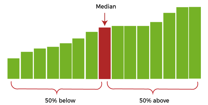

History

Scientists in the ancient Near East did not only employ summary statistics, instead selecting numbers that showed the greatest agreement with a more general theory that included a range of occurrences. Statistics like the mean are a mediaeval and early modern creation within the Mediterranean (and, subsequently, European) academic community.

In order to objectively analyse disparate assessments, the concept of the median first appears in the Talmud in the sixth century. The idea, meanwhile, needed to catch on with the larger scientific community.

Instead, Al-Biruni's invention of the mid-range serves as the present median's closest predecessor. It is still being determined how Al-Biruni's work was passed on to succeeding academics. Al-Biruni used his method to assay metals, but even after he published his findings, the majority of assayers continued to choose the least favourable value from their results out of concern that it would make them look to be cheating. However, when maritime transportation developed throughout the Age of Discovery, ship navigators were forced to make more attempts to calculate latitude in unfavourable weather and against unfriendly coasts, which sparked a resurgence in interest in summary statistics. Whether it was independently created or found, Harriot's "Instructions for Raleigh's Voyage to Guiana, 1595" advises marine navigators to use the mid-range.

The concept of the median may have originally appeared in a section on compass navigation in Edward Wright's 1599 book Certaine Errors in Navigation. Since the median included a larger part of the information than the mid-range, Wright may have concluded that it was more likely to be accurate since he was hesitant to throw out measured numbers. However, it is difficult to confirm if Wright accurately characterised the present concept of median since he did not provide instances of how his approach was used. The median (in the context of probability) was mentioned in Christiaan Huygens' letter but as an illustration of a statistic that wasn't suitable for use in actuarial practice.

The L1 norm and, indirectly, the median was the foundations of Roger Joseph Boscovich's regression approach, which was the first to advocate the median. This was in 1757. Laplace made this wish clear in 1774 when he proposed using the median as the accepted estimator of the value of a posterior PDF. The precise standard was |alpha -alpha *|, where alpha * is the estimate and alpha is the real value, to minimise the predicted amount of the mistake. Laplace established the distributions of the sample mean and sample median in the early 1800s in order to achieve this. But a decade later, Gauss and Legendre created the least squares approach, which gets the mean by minimising (alpha -alpha *)². The invention of Gauss and Legendre allows much simpler computing in the area of regression. Laplaces' suggestion was hence often disregarded until the development of computer technology 150 years later (and is still a rather unusual approach).

The word median (valeur m�diane), which refers to the value that splits a probability distribution into two halves, was originally used by Antoine Augustin Cournot in 1843. The median (Centralwerth) was employed by Gustav Theodor Fechner to analyse social and psychological phenomena. It had previously exclusively been used for astronomy and associated subjects. Although Laplace had previously used it, and the median had been mentioned in a textbook by F. Y. Edgeworth, it was Gustav Fechner who made the median widely employed in the formal analysis of data. Following the introduction of the phrases middle-most value in 1869 and medium in 1880, Francis Galton first used the English term median in that year.

Throughout the 19th century, statisticians heavily promoted the usage of medians due to their intuitive clarity and simplicity in manual calculation. The idea of the median, however, is far more difficult to calculate by computer and does not lend itself to the theory of higher moments as well as the arithmetic mean does. As a consequence, over the 20th century, the arithmetic mean gradually replaced the median as a concept of general average.

Finite Data Set of Numbers

When a finite list of integers is arranged from least to biggest, the median is the "middle" number.

The middle observation is chosen if the data collection has an odd number of observations. The following list includes seven numbers, for instance

The median value for the numbers 1, 3, 3, 6, 7, 8, and 9 is 6, the fourth value.

When there are exactly equal numbers of observations in the data set, there is no clear middle value, and the median is often the arithmetic mean of the two middle values. For instance, this collection of 8 digits

1, 2, 3, 4, 5, 6, 8, and 9 all have a median value 4.5. This reads the median as the completely trimmed mid-range (in more technical words).

Generally speaking, the median may be defined as follows using this convention: When n items in a data collection x are sorted from least to biggest,

If n is odd, median(x) = x_(n+1)/2

If n is even, median(x) = x_(n/2)+ x_((n/2)+1)/ 2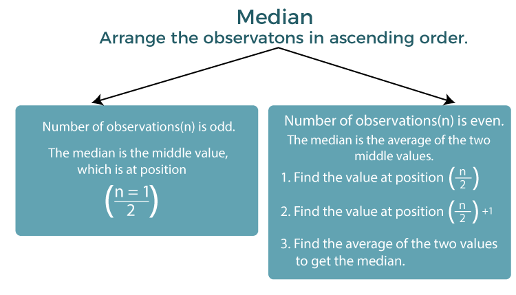

Formal Definition

Formally, the median of a population is any figure where at least half of the population is more than or equal to the proposed median and at least half is less than the proposed median. As was already said, medians could not be special. If more than half of the population is present in each set, then a portion of the population is precisely equal to the different median. Any ordered (one-dimensional) data set has a well-defined median that is unaffected by any distance measure. Thus, the median may be used in classes that are ranked but not numerical (e.g., calculating a median grade when students are given grades from A to F). Yet, the outcome can be in the middle of the classes if there are an even number of instances.

On the other hand, a geometric median may be specified in as many dimensions as desired. The medoid is a similar idea in which the result is made to match a sample participant. Although there isn't a universally recognised standard notation for the median, some writers choose to write the median of a variable x as either x or x_1/2, sometimes also as M. Any of these instances require that the median's usage of these symbols, or any other symbols, be presented with a clear definition. The median is a specific case of the second quartile, fifth decile, and 50th percentile to summarise the usual values associated with a statistical distribution.

Uses

The median may be used as a measure of location when one gives less weight to extreme values. It is generally because the distribution is skewed, the values at the extremes are unknown, or outliers are unreliable, i.e., they might be transcription or measurement mistakes.

Take the multiset as an example:

1, 2, 2, 2, 3, 14.

In this instance, the mode and median are both 2; these numbers may be seen as more representative of the centre than the arithmetic mean, which is 4 in this instance and bigger than all but one of the values. The commonly accepted empirical connection, according to which the mean is "further into the tail" of a distribution than the median, is not always accurate. At best, one may assert that the two statistics cannot be "too far" apart; for further information, read the section below on inequality-related means and medians.

It is optional to know the value of the extreme outcomes in order to determine a median since it is based on the middle data in a collection. A median may still be derived, for instance, if a tiny percentage of respondents failed to solve the issue at all within the allotted time in a psychological test assessing the length of time required to answer a problem.

The median is a common summary statistic in descriptive statistics because it is clear to comprehend, simple to compute, and provides a reliable approximation to the mean. There are various options for a measure of variability in this situation, including the range, interquartile range, mean absolute deviation, and median absolute deviation.

Practical comparisons between various location and dispersion measurements often centre on how effectively the related population values may be inferred from a sample of data. The median's attributes are excellent when calculated using the sample median. If a certain population distribution is adopted, it could be better, but its features are always respectably decent. The sample mean, for instance, is statistically more efficient when?and only when?data are free of data from mixes of distributions or from heavy-tailed distributions, according to a comparison of the efficiency of candidate estimators. However, the median still outperforms the minimum-variance mean (64% efficiency for large normal samples), which means that the variance of the median will be around 50% higher than the variance of the mean.

Medians of Certain Distributions

Even for certain distributions without a clearly defined mean, such as the Cauchy distribution, the medians of some kinds of distributions may be computed from their parameters:

A symmetric unimodal distribution has a median that is equal to its mode.
A symmetric distribution with a mean also has a value in its median.
A normal distribution with a mean of 1 and a variance of 2 has a median value of 1. In actuality, mean equals median = mode for a normal distribution.
In the range [a, b], the median of a uniform distribution is equal to (a + b) / 2, which is also the mean.
The location parameter, denoted by x₀, serves as the median of a Cauchy distribution with scale and location parameters, respectively.
The minimal value for which the power law holds is x_min, and the median of a power law distribution with exponent a > 1 is 21/(a₁)x_min.
The ratio of the natural logarithm of 2 to the rate parameter, or ¹ln₂, is the value of the median in an exponential distribution with the rate parameter.
(ln 2)^1/k is the median of a Weibull distribution with shape parameter k and scaling parameter.

Properties

Property of optimality

E(|X-c|)

is the mean absolute error between a real variable c and a random variable X.

If the probability distribution of X allows for the existence of the expectation as mentioned earlier, then m is the median of X if and only if m minimises the mean absolute error relative to X. Specifically, it minimises the arithmetic mean of the absolute deviations if m is a sample median. But keep in mind that this minimiser is not exclusive when the sample has an even number of components.

A median is more broadly described as a minimum of:

E(|X-c|-|X|),

as is covered in the section on multivariate medians (more particularly, the spatial median) below.

This median definition based on optimisation is helpful for analysing statistical data, such as when clustering k-medians.

Unfairness Involving Means and Medians

Comparison of the means, medians, and modes of two distributions of logarithms with varying skewness. The difference between the median and mean in a distribution with finite variance is constrained to one standard deviation.

For discrete samples, this limit was established by Book and Sher in 1979 and more extensively by Page and Murty in 1982. As a remark on a later demonstration by O'Cinneide, Mallows, in 1991, offered a brief demonstration that twice makes use of Jensen's inequality. When we use || as the absolute value, we get:

I μ - m I =I E(X - m)I </= E(IX - mI)

</= E(IX - μ I)

</= under root E (( X - μ )²) = σ

The first and third inequalities result from applying Jensen's inequality to the square function and the absolute-value function, both of which are convex functions. A median reduces the absolute deviation function a � E(I X - a I), which leads to the second inequality.

By simply substituting a norm for the absolute value in Mallows's argument, a multivariate version of the inequality may be obtained:

II μ - m II </ = under root E ( II X - μ II²) = under root trace ( var (X))

When m is a function minimiser a� E ( II X - a II), or a spatial median when the data set has two or more dimensions, the spatial median is distinct.

The one-sided Chebyshev inequality, which may be found in an inequality on location and scale parameters, is used in an alternate proof. Additionally, Cantelli's inequality immediately leads to this formula.

Medians for samples

Effective sample median calculation

Despite the fact that comparison-sorting n items needs (n log n) operations, selection algorithms may determine which item is the kth-smallest from n with only (n) operations. Included in this is the median, which is the n/2nd order statistic (or, for even numbers of samples, the arithmetic mean of the two middle-order statistics).

The drawback of selection algorithms is that they still require (n) memory; that is, they need to store the whole sample in memory (or a linear-sized piece of it). There are numerous methods for estimating the median because of this, as well as the linear time required, which may be prohibitive. The quicksort sorting algorithm often employs the median of three rules as a subroutine, which estimates the median as the median of a three-element subsample. This rule is straightforward and uses an estimate of the input's median. Tukey's ninther, which is the median of three rules applied with little recursion, is a more reliable estimator: if A is an array representing the sample, and

med3 (A) = median(A[1],A[n/2],A[n]),

then

ninether(A) = med3(med3(A[1.....1n/3]), med3(A[1n/3.....2n/3]), med3(A[2n/3.....n]))

The remedian is an estimator for the median that operates in a single pass over the sample and has linear time but sub-linear memory requirements.

Sampling Distribution

Laplace was used to calculate the distributions of the sample median and mean. Asymptotically normal with menu mu and variance, the distribution of the sample median from a population with a density function f(x) where

1/4nf( m)²

where median m is f(x), and the sample size is n.

sample median ~ N ( μ = m , σ²= 1/4nf( m)²

The following is contemporary proof. It is now known that Laplace's finding is a specific instance of the asymptotic distribution of arbitrary quantiles.

The density is normal samples, where the density is f(m) = 1 / under root 2π σ²

hence, for large samples, the median's variance equals ( π/2)*( σ²/n).

The Asymptotic Distribution's Deviation

The formula for the case of discrete variables is provided below in Empirical local density. We assume our variable is continuous and the sample size is an odd number. The sample may be summarised as "below median", "at median", and "above median," which corresponds to a trinomial distribution with probability.

Since several sample values for a continuous variable can't be precisely equal to the median, the density at point v may be calculated directly from the trinomial distribution:

Pr [ Median = v] dv = (2n + 1)! / n! n! . F (v)ⁿ(1-F(v))ⁿ f (v) dv

We'll now discuss the beta function. When using integer parameters α and β can be expressed as

B ( α , β ) = ( α -1) ! (β - 1) !/ ( α + β - 1 )!

Also, f (v) dv = dF(v),

Using these connections and establishing both α and β equal to n+1 can also be written as

F (v)ⁿ(1-F(v))ⁿ/ B(n+1, n+1) dF(v)

Consequently, the median density function is a symmetric beta distribution that has been advanced by F. Its variance is equal to its mean, which is 0.5, as expected.

According to the chain rule, the sample median's associated variance is

1/ 4 (N+2)f(m)²

The extra two hardly count towards the limit.

Median Across Several Variables

When the sample or population had only one dimension, the univariate median was explained in a previous section of this article. There are many ideas that go beyond the definition of the univariate median when the dimension is two or higher; each of these multivariate medians agrees with the univariate median when the dimension is precisely one.

Median Margin

For vectors specified with respect to a predetermined set of coordinates, the marginal median is defined. A vector whose elements are univariate medians is referred to as a marginal median. The features of the marginal median have been researched by Puri and Sen, and it is simple to calculate.

Geometric Median

The point that minimises the sum of distances to the sample points is the geometric median of a discrete collection of sample points x₁,... x₂in Euclidean space.

The geometric median is equivariant with regard to Euclidean similarity transformations, such as translations and rotations, in contrast to the marginal median.

All Directions' Median

The "median in all directions" is the position where the marginal medians for all coordinate systems meet. Because of the median voter theorem, this idea has application to voting theory. The geometric median, when it exists (at least for discrete distributions), corresponds with the median in all directions.